Heading-aware kernel density

Computes an approximate density useful for visualization. For proper circular densities, use hdg_circular() and circular::density.circular().

hdg_density(
  hdg,
  bw = 5,
  kernel = c("gaussian", "epanechnikov", "rectangular", "triangular", "biweight",
    "cosine", "optcosine"),
  weights = NULL,
  n = 512,
  na.rm = FALSE,
  ...
)

# S3 method for hdg_density
plot(x, main = NULL, xlab = NULL, ylab = NULL, axes = TRUE, ...)

hdg_plot(
  hdg,
  density = hdg_density(hdg, na.rm = TRUE),
  main = NULL,
  xlab = NULL,
  ylab = NULL,
  axes = TRUE,
  ...
)

Arguments

hdg	A heading in degrees, where 0 is north, 90 is east, 180 is south, and 270 is west. Values outside the range [0-360) are coerced to this range using hdg_norm().
bw	The bandwidth of the smoothing kernel. Automatic methods are not available, so you will have to set this value manually to obtain the smoothness you want.
kernel	a character string giving the smoothing kernel to be used. This must partially match one of "gaussian", "rectangular", "triangular", "epanechnikov", "biweight", "cosine" or "optcosine", with default "gaussian", and may be abbreviated to a unique prefix (single letter). "cosine" is smoother than "optcosine", which is the usual ‘cosine’ kernel in the literature and almost MSE-efficient. However, "cosine" is the version used by S.
weights	numeric vector of non-negative observation weights, hence of same length as x. The default NULL is equivalent to weights = rep(1/nx, nx) where nx is the length of (the finite entries of) x[].
n	the number of equally spaced points at which the density is to be estimated. When n > 512, it is rounded up to a power of 2 during the calculations (as fft is used) and the final result is interpolated by approx. So it almost always makes sense to specify n as a power of two.
na.rm	logical; if TRUE, missing values are removed from x. If FALSE any missing values cause an error.
...	For hdg_density(), dots are unused; for plot.hdg_density(), dots are passed to graphics::lines(); for hdg_plot(), passed to graphics::points()
x	the data from which the estimate is to be computed. For the default method a numeric vector: long vectors are not supported.
main, xlab, ylab, axes	See graphics::plot().
density	A hdg_density() object.

Value

An object identical to stats::density() but with class "hdg_density".

Examples

x <- head(kamloops2016$wind_dir, 1000)
hdg_density(x, na.rm = TRUE)
#> 
#> Call:
#> 	hdg_density(hdg = x, na.rm = TRUE)
#> 
#> Data: x (512 obs.);	Bandwidth 'bw' = 5
#> 
#>        x             y           
#>  Min.   :  0   Min.   :0.000000  
#>  1st Qu.: 90   1st Qu.:0.000000  
#>  Median :180   Median :0.000000  
#>  Mean   :180   Mean   :0.002797  
#>  3rd Qu.:270   3rd Qu.:0.000000  
#>  Max.   :360   Max.   :0.046648  
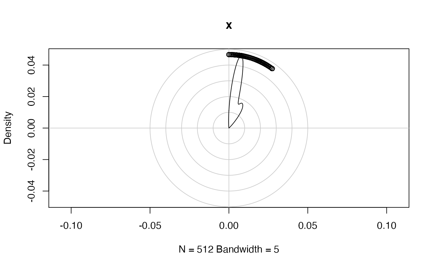
plot(hdg_density(x, na.rm = TRUE))
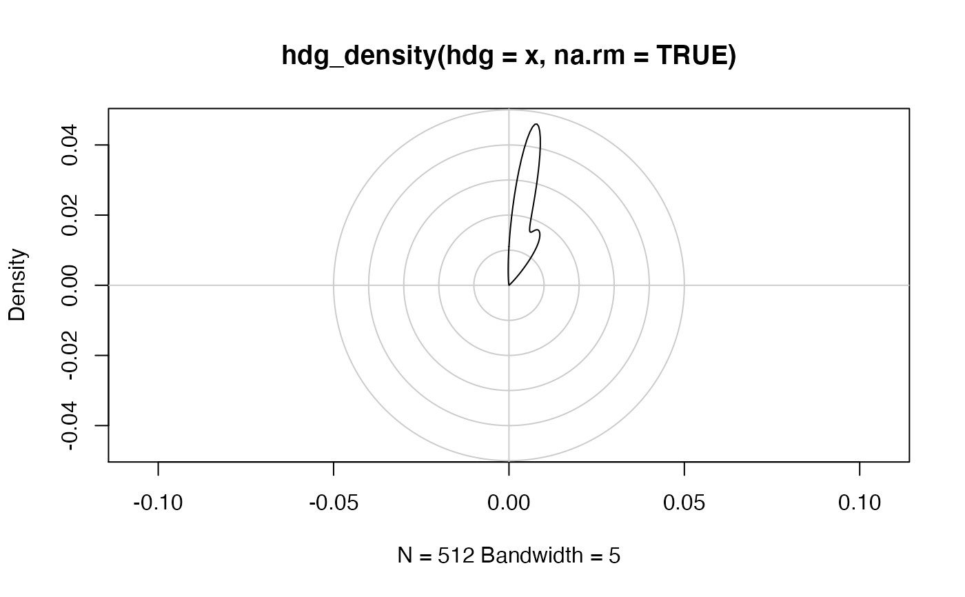hdg_plot(x)