Rclimateca
An R Package to fetch climate data from Environment Canada
rclimateca
Fetching data from Environment Canada's archive has always been a bit of a chore. In the old days, it was necessary to download data one click at a time from the organization's search page. To bulk download hourly data would require a lot of clicks and a good chance of making a mistake and having to start all over again. There are several R solutions online (posted by Headwater Analytics and From the Bottom of the Heap ), but both solutions are mostly single-purpose, and don't solve the additional problem of trying to find climate locations near you. In the rclimateca package, I attempt to solve both of these problems to produce filtered, plot-ready data from a single command.
Installation
Rclimateca is available on CRAN and can be installed using the install.packages().
install.packages('rclimateca')Finding climate stations
We will start with finding sites near where you're interested in. Sometimes you will have a latitude and longitude, but most times you will have a town or address. Using the prettymapr packages 'geocode' function, the getClimateSites() function looks up locations near you.
library(rclimateca)
getClimateSites("gatineau QC")
## Name Province Station ID Latitude (Decimal Degrees)
## 5648 OTTAWA CITY HALL ONTARIO 4334 45.43
## 5654 OTTAWA LA SALLE ACAD ONTARIO 4339 45.43
## 5656 OTTAWA LEMIEUX ISLAND ONTARIO 4340 45.42
## 5663 OTTAWA U OF O ONTARIO 4346 45.42
## 5662 OTTAWA STOLPORT A ONTARIO 7684 45.47
## Longitude (Decimal Degrees) First Year Last Year
## 5648 -75.70 1966 1975
## 5654 -75.70 1954 1967
## 5656 -75.73 1953 1979
## 5663 -75.68 1954 1955
## 5662 -75.65 1974 1976
If you also need data for a set of years, you can also pass a vector of years to further refine your data.
getClimateSites("gatineau QC", year=2014:2016)## Name Province Station ID Latitude (Decimal Degrees)
## 7147 CHELSEA QUEBEC 5585 45.52
## 5646 OTTAWA CDA ONTARIO 4333 45.38
## 5647 OTTAWA CDA RCS ONTARIO 30578 45.38
## 7154 OTTAWA GATINEAU A QUEBEC 50719 45.52
## 7155 OTTAWA GATINEAU A QUEBEC 53001 45.52
## Longitude (Decimal Degrees) First Year Last Year
## 7147 -75.78 1927 2016
## 5646 -75.72 1889 2016
## 5647 -75.72 2000 2016
## 7154 -75.56 2012 2016
## 7155 -75.56 2014 2016
If you'd like to apply your own subsetting operation, the entire dataset is also available through this package (although it may be slightly out of date).
data("climateLocs2016")
names(climateLocs2016)
## [1] "Name" "Province"
## [3] "Climate ID" "Station ID"
## [5] "WMO ID" "TC ID"
## [7] "Latitude (Decimal Degrees)" "Longitude (Decimal Degrees)"
## [9] "Latitude" "Longitude"
## [11] "Elevation (m)" "First Year"
## [13] "Last Year" "HLY First Year"
## [15] "HLY Last Year" "DLY First Year"
## [17] "DLY Last Year" "MLY First Year"
## [19] "MLY Last Year"
Downloading data
Downloading data is accomplished using the getClimateData() function, or if you'd like something less fancy, the getClimateDataRaw() function. There is documentation in the package for both, but getClimateData() has all the bells and whistles, so I will go over its usage first. You will first need a stationID (or a vector of them) - in our case I'll use the one for Chelsea, QC, because I like the ice cream there.
df <- getClimateData(5585, timeframe="daily", year=2015)
str(df)
## 'data.frame': 365 obs. of 29 variables:
## $ stationID : num 5585 5585 5585 5585 5585 ...
## $ Date/Time : chr "2015-01-01" "2015-01-02" "2015-01-03" "2015-01-04" ...
## $ Year : int 2015 2015 2015 2015 2015 2015 2015 2015 2015 2015 ...
## $ Month : int 1 1 1 1 1 1 1 1 1 1 ...
## $ Day : int 1 2 3 4 5 6 7 8 9 10 ...
## $ Data Quality : logi NA NA NA NA NA NA ...
## $ Max Temp (°C) : num NA NA NA NA -16.5 NA NA -10.5 -6.5 NA ...
## $ Max Temp Flag : chr "M" "M" "M" "M" ...
## $ Min Temp (°C) : num NA NA NA NA NA -26 -24.5 -31.5 -20.5 NA ...
## $ Min Temp Flag : chr "M" "M" "M" "M" ...
## $ Mean Temp (°C) : num NA NA NA NA NA NA NA -21 -13.5 NA ...
## $ Mean Temp Flag : chr "M" "M" "M" "M" ...
## $ Heat Deg Days (°C) : num NA NA NA NA NA NA NA 39 31.5 NA ...
## $ Heat Deg Days Flag : chr "M" "M" "M" "M" ...
## $ Cool Deg Days (°C) : num NA NA NA NA NA NA NA 0 0 NA ...
## $ Cool Deg Days Flag : chr "M" "M" "M" "M" ...
## $ Total Rain (mm) : num NA NA NA NA 0 0 0 0 0 0 ...
## $ Total Rain Flag : chr "M" "M" "M" "M" ...
## $ Total Snow (cm) : num NA NA NA NA 0.3 6.2 0.5 2.6 0 NA ...
## $ Total Snow Flag : chr "M" "M" "M" "M" ...
## $ Total Precip (mm) : num NA NA NA NA 0.3 6.2 0.5 2.6 0 NA ...
## $ Total Precip Flag : chr "M" "M" "M" "M" ...
## $ Snow on Grnd (cm) : int NA NA NA NA 14 14 18 16 17 17 ...
## $ Snow on Grnd Flag : chr "M" "M" "M" "M" ...
## $ Dir of Max Gust (10s deg): logi NA NA NA NA NA NA ...
## $ Dir of Max Gust Flag : logi NA NA NA NA NA NA ...
## $ Spd of Max Gust (km/h) : logi NA NA NA NA NA NA ...
## $ Spd of Max Gust Flag : logi NA NA NA NA NA NA ...
## $ parsedDate : POSIXct, format: "2015-01-01" "2015-01-02" ...
Boom! Data! The package can also melt the data for you (à la reshape2) so that you can easily use ggplot to visualize.
library(ggplot2)
df <- getClimateData(5585, timeframe="daily", year=2015, format="long")
ggplot(df, aes(parsedDate, value)) + geom_line() +
  facet_wrap(~param, scales="free_y")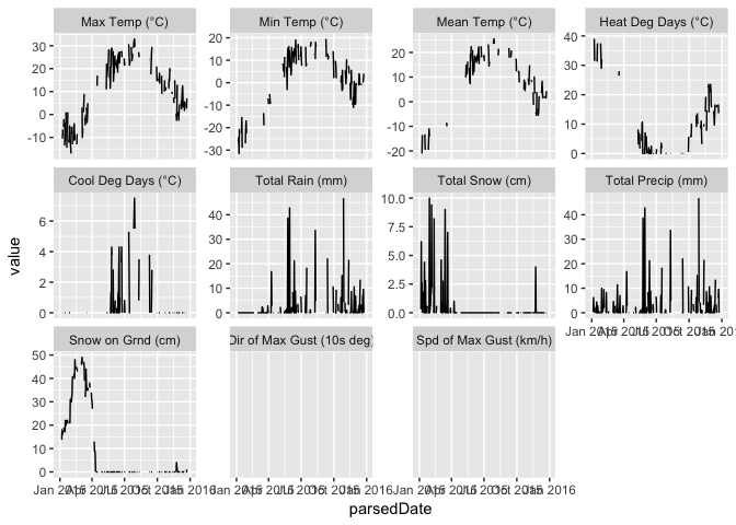
The function can accept a vector for most of the parameters, which it uses to either download multiple files or to trim the output, depending on the parameter. How to Chelsea, QC and Kentville, NS stack up during the month of November (Pretty similar, as it turns out...)?
df <- getClimateData(c(5585, 27141), timeframe="daily", year=2015, month=11, format="long")
ggplot(df, aes(parsedDate, value, col=factor(stationID))) +
  geom_line() + facet_wrap(~param, scales="free_y")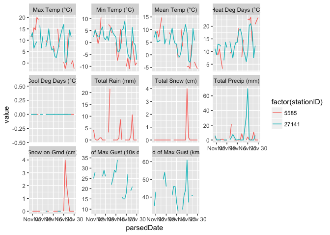
You will also notice that a little folder called ec.cache has popped up in your working directory, which contains the cached files that were downloaded from the Environment Canada site. You can disable this by passing cache=NULL, but I don't suggest it, since the cache will speed up running the code again (not to mention saving Environment Canada's servers) should you make a mistake the first time.
This function can download a whole lot of data, so it's worth doing a little math for yourself before you overwhelm your computer with data that it can't all load into memory. As an example, I tested this function by downloading daily data for every station in Nova Scotia between 1900 and 2016, which took 2 hours, nearly crashed my compute,r and resulted in a 1.3 gigabyte data.frame. You can do a few things (like ensure checkdate=TRUE and, if you're using format="long", rm.na=T) to make your output a little smaller, or you can pass ply=plyr::a_ply to just cache the files so you only have to download them the once.
A little on how it works
The code behind this package is available on GitHub, but it is fairly extensive and designed to tackle all of the corner cases that make writing a package so much more difficult than a script that runs once. Essentially, it's very close to the solution posted on From the Bottom of the Heap and in the documentation itself. From the documentation:
for year in `seq 1998 2008`;do for month in `seq 1 12`;do wget --content-disposition "http://climate.weather.gc.ca/climate_data/bulk_data_e.html?format=csv&stationID=1706&Year=${year}&Month=${month}&Day=14&timeframe=1&submit= Download+Data" ;done;done

WHERE;
 year = change values in command line (`seq 1998 2008)
 month = change values in command line (`seq 1 12)
 format= [csv|xml]: the format output
 timeframe = 1: for hourly data
 timeframe = 2: for daily data
 timeframe = 3 for monthly data
 Day: the value of the "day" variable is not used and can be an arbitrary value
 For another station, change the value of the variable stationID
 For the data in XML format, change the value of the variable format to xml in the URL.
This is, of course, the same as the genURLS() solution except for bash and wget instead of for R. This package uses the "format=csv" option, which produces a somewhat malformed CSV (there is quite a bit of header information). The "guts" of the read operation are as follows:
# download the file
library(httr)
url <- "http://climate.weather.gc.ca/climate_data/bulk_data_e.html?format=csv&stationID=1706&Year=2008&Month=5&Day=14&timeframe=1&submit=Download+Data"
connect <- GET(url)
x <- content(connect, as="text", encoding="UTF-8")

# find the second emtpy line and start the read.csv after that line
xlines <- readLines(textConnection(x))
empty <- which(nchar(xlines) == 0)
empty <- empty[empty != length(xlines)]
# read the data frame
df <- read.csv(textConnection(x),
               skip=empty[length(empty)],
               stringsAsFactors = F, check.names = F)
I am sure is cringing as I read the entirity of each CSV file into memory, but they should be reminded that (a) R is terrible for memory usage anyway, and (b) the files are already "chunked up" by Environment Canada so that there is no chance of getting an unwieldy-sized file by accident.
Wrapping it up
That's it! Hopefully now you can all download unlimited quantities of data in pure bliss (as long as Environment Canada keeps its URLs consistent).