grd() objects are just an array (any object with more than
two dim()s) and a bounding box (a rct(), which may or
may not have a wk_crs() attached). The ordering of the dimensions
is y (indices increasing downwards), x (indices increasing to the right).
This follows the ordering of as.raster()/rasterImage() and aligns
with the printing of matrices.
grd(
  bbox = NULL,
  nx = NULL,
  ny = NULL,
  dx = NULL,
  dy = NULL,
  type = c("polygons", "corners", "centers")
)

grd_rct(data, bbox = rct(0, 0, dim(data)[2], dim(data)[1]))

grd_xy(data, bbox = rct(0, 0, dim(data)[2] - 1, dim(data)[1] - 1))

as_grd_rct(x, ...)

# S3 method for class 'wk_grd_rct'
as_grd_rct(x, ...)

# S3 method for class 'wk_grd_xy'
as_grd_rct(x, ...)

as_grd_xy(x, ...)

# S3 method for class 'wk_grd_xy'
as_grd_xy(x, ...)

# S3 method for class 'wk_grd_rct'
as_grd_xy(x, ...)
Arguments
- bbox
A
rct()containing the bounds and CRS of the object. You can specify arct()withxmin > xmaxorymin > ymaxwhich will flip the underlying data and return an object with a normalized bounding box and data.- nx, ny, dx, dy
Either a number of cells in the x- and y- directions or delta in the x- and y-directions (in which case
bboxmust be specified).- type
Use "polygons" to return a grid whose objects can be represented using an
rct(); use "centers" to return a grid whose objects are the center of therct()grid; use "corners" to return a grid along the corners ofbbox.- data
An object with two or more dimensions. Most usefully, a matrix.
- x
An object to convert to a grid
- ...
Passed to S3 methods
Value
grd()returns agrd_rct()fortype == "polygonsor agrd_xy()otherwise.grd_rct()returns an object of class "wk_grd_rct".grd_xy()returns an object of class "wk_grd_xy".
Examples
# create a grid with no data (just for coordinates)
(grid <- grd(nx = 2, ny = 2))
#> <wk_grd_rct [2 x 2 x 0] => [0 0 2 2]>
#> List of 2
#> $ data: logi[1:2, 1:2, 0 ]
#> $ bbox: wk_rct[1:1] [0 0 2 2]
#> - attr(*, "class")= chr [1:2] "wk_grd_rct" "wk_grd"
as_rct(grid)
#> <wk_rct[4]>
#> [1] [0 1 1 2] [0 0 1 1] [1 1 2 2] [1 0 2 1]
as_xy(grid)
#> <wk_xy[4]>
#> [1] (0.5 1.5) (0.5 0.5) (1.5 1.5) (1.5 0.5)
plot(grid, border = "black")
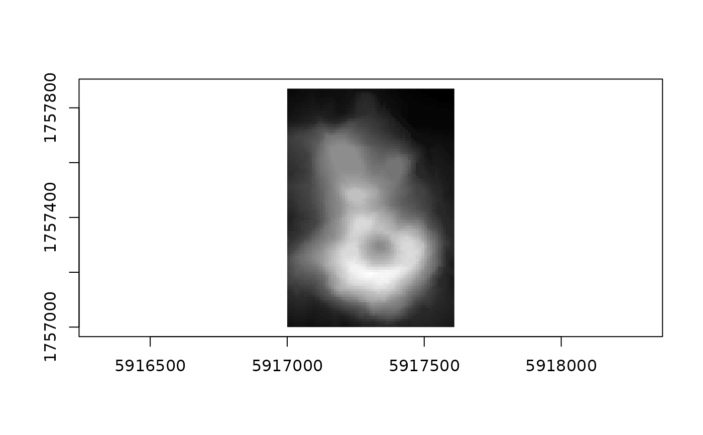
 # more usefully, wraps a matrix or nd array + bbox
# approx volcano in New Zealand Transverse Mercator
bbox <- rct(
5917000, 1757000 + 870,
5917000 + 610, 1757000,
crs = "EPSG:2193"
)
(grid <- grd_rct(volcano, bbox))
#> <wk_grd_rct [87 x 61] => [5917000 1757000 5917610 1757870] with crs=EPSG:2193>
#> List of 2
#> $ data: num [1:87, 1:61] 97 97 98 98 99 99 99 99 100 100 ...
#> $ bbox: wk_rct[1:1] [5917000 1757000 5917610 1757870]
#> - attr(*, "class")= chr [1:2] "wk_grd_rct" "wk_grd"
# these come with a reasonable default plot method for matrix data
plot(grid)
# more usefully, wraps a matrix or nd array + bbox
# approx volcano in New Zealand Transverse Mercator
bbox <- rct(
5917000, 1757000 + 870,
5917000 + 610, 1757000,
crs = "EPSG:2193"
)
(grid <- grd_rct(volcano, bbox))
#> <wk_grd_rct [87 x 61] => [5917000 1757000 5917610 1757870] with crs=EPSG:2193>
#> List of 2
#> $ data: num [1:87, 1:61] 97 97 98 98 99 99 99 99 100 100 ...
#> $ bbox: wk_rct[1:1] [5917000 1757000 5917610 1757870]
#> - attr(*, "class")= chr [1:2] "wk_grd_rct" "wk_grd"
# these come with a reasonable default plot method for matrix data
plot(grid)
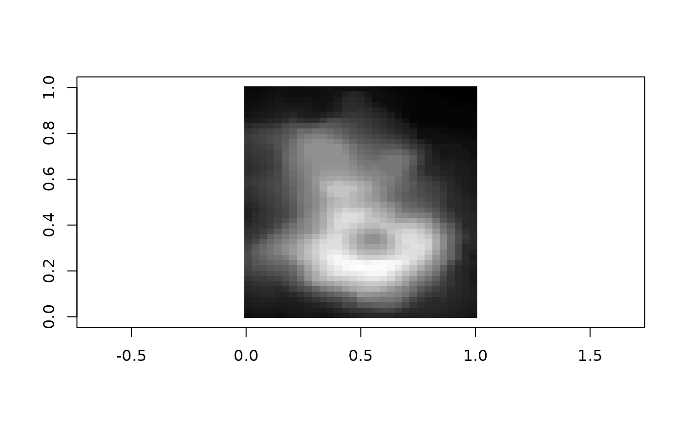
 # you can set the data or the bounding box after creation
grid$bbox <- rct(0, 0, 1, 1)
# subset by indices or rct
plot(grid[1:2, 1:2])
# you can set the data or the bounding box after creation
grid$bbox <- rct(0, 0, 1, 1)
# subset by indices or rct
plot(grid[1:2, 1:2])
 plot(grid[c(start = NA, stop = NA, step = 2), c(start = NA, stop = NA, step = 2)])
 plot(grid[rct(0, 0, 0.5, 0.5)])