Open Street Map Data in R

The Open Street Map project is an incredible resource for those interested in accessing worldwide geographic data, which is often as good or better than that provided by Google Maps. In addition to providing pre-rendered tiles that are acessible on the web, in R, or in QGIS, Open Street map provides access to the raw data used to create its maps. In R, this package takes the form of the osmar package.

Recently I submitted a proposal on Upwork to compare GPS tracks collected from Android phones to Open Street Map data to see which tracks were from a highway and which were not. Before submitting, I tested the waters of Open Street Map data in R just to see what was possible. What I wanted to do was:

Download OSM data for a given bouding box
Extract highway data
Given a lat/lon, find the nearest highway

The Packages

I always try to keep the packages used to a minimum, but here there's a few that are necessary to keep the amount of code to a minimum. The most important is the osmar package, but I'll also use prettymapr and geosphere for a few helpful functions.

library(osmar) # (geosphere is inclued in osmar)
library(prettymapr)

Getting OSM Data

To retreive OSM data via the Open Street Map API, all we need to do is call the get_osm() function with a bounding box as the argument. osmar has its own lingo for describing a bounding box, so you're best off using its own methods for creating one: center_bbox(lon, lat, width, height) (where width and height are in metres) or corner_bbox(). I personally can't be bothered to type in coordinates when there's an entire internet making it so I don't have to, so I'm going to use the searchbbox function from the prettymapr package and convert the results manually:

wolfville <- searchbbox("wolfville, ns", 
                              source="google")
wolfville <- c(wv[1], wv[2], wv[3], wv[4])
names(wolfville) <- c("left", "bottom", 
                                "right", "top")
class(wolfville) <- "bbox"

After that, getting the data is easy:

osmdata <- osmar::get_osm(wolfville)

The osmdata contains an osmar object, which has all the 'nodes' and 'ways' associated with the data. To get a 'flat' view of the data, try: osmdata$nodes$attrs or osmdata$nodes$tags, which are data.frame objects that store data associated with each node. Similarly, osmdata$ways$attrs and osmdata$ways$tags store information about each 'way'. You can also plot_ways(osmdata) and plot_nodes(osmdata) to see what they look like on a map.

Extract Highway Data

There's lots of data other than roads in our osmdata object, so we need to subset the data such that we only have data associated with the roads. There's an example of this in the vignette published by osmar authors, which we'll adapt to our purposes.

hways_data <- subset(osmdata, 
                way_ids = find(osmdata, 
                  way(tags(k == "highway"))))
hways <- find(hways_data, way(tags(k == "name")))
hways <- find_down(osmdata, way(hways))
hways_data <- subset(osmdata, ids = hways)

I'm still not entirely sure what this does, but it uses the subset and find methods to get any 'way' (line) that has a tag 'highway' and tag 'name'. Then, it uses the find_down() function to get the ways and the 'nodes' associated with these 'ways'. Getting used to the 'node' and 'ways' syntax used by osmar takes a while, but the basic idea is that a 'way' is made up of several 'nodes'. The find_up() function will take a node id and find the way it is associated with (if there is one), while the find_down() function will take a way and find the nodes associated with it. Anytime you pass an ID to find(), find_up(), or find_down() you have to specify using way() or node() which type of feature you mean. Using the tags() function is a way to select nodes or ways that have a key (k=) and/or value ( v=). The exact syntax for this I'm not exactly sure of, but it's not explained particularly well in the manual so I thought I'd give the basics here.

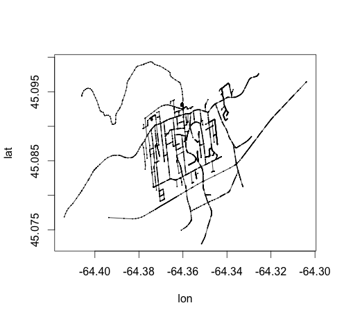
The osmar package provides some functions to visualize nodes and ways, notably plot_nodes() and plot_ways(). If we call both on our data, we can get a preview of what we just did:

plot_ways(hways_data)
plot_nodes(hways_data, pch=19, cex=0.1, add=T)

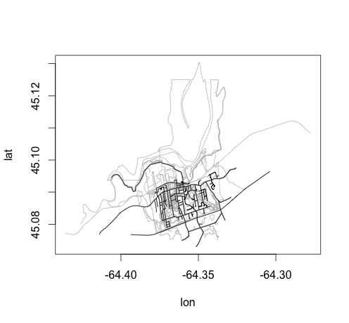
Let's compare this to our original data by plotting the original data in gray.

plot_ways(osmdata, col="gray")
plot_ways(hways_data, add=T)

Finding the nearest highway

Now we have a complete inventory of all the roads in our dataset, so the next step is to build a function that, given a lat/lon point, finds the nearest 'node', and then use the find_up() function to find the 'way' associated with that 'node'. Then, we can search the 'tags' to find the name of that road. Intimidated? It's easier broken down into a few steps.

Let's start with the 'nearest node' bit. The lat and lon of each node can be found in the hways_data$nodes$attrs data frame.

hway_nodes_attrs <- hways_data$nodes$attrs
lons <- hway_nodes_attrs$lon
lats <- hway_nodes_attrs$lat

Now if we define our point, we can create a distance matrix using the distm() function in the package geosphere (which is already loaded for us by osmar). If you're looking to find a point without typing (did I mention how much I hate typing?), try locator(n=1).

point <- c(-64.37712, 45.0862)
distances <- distm(cbind(lons, lats), point)

Now we can use which.min() to find the row with the minimum distance, and use our hway_nodes_attrs data frame to find the ID of that node.

row <- which.min(distances)
node_id <- hway_nodes_attrs$id[row]

Next we'll use the find_up() method to find the 'way' associated with that 'node'. It's worth noting that find_up() is fully vectorized, so if you put in a vector of node ids then you'll get a vector of way ids back (which you may want to do if you're looking for the closest n points instead of just a single node, for example).

waydata <- find_up(hways_data, node(node_id))
waydata$way_ids # == 83765582, in this example

To get the 'tags' associated with that, we'll subset() the hways_data object according to way_ids.

nearest_way <- subset(hways_data, 
                     way_ids = waydata$way_ids)
nearest_way_tags <- nearest_way$ways$tags
nearest_way_tags$v[nearest_way_tags$k=="name"]

In this case, our answer should be Stirling Avenue, which seems reasonable. Note that we can't plot_ways(nearest_way) because we didn't include any of the nodes when subsetting the data. For an example of this, look at where we subetted the osmdata object in the first step, where we had to use find_down() to get the 'nodes' associtated with the 'ways' that were tagged "highway". It's a complicated game, but a powerful one if you can wrap your mind around it.

A cool way to visualize this is to use the locator() function in a loop to do this a bunch of times (in this case you'll have to hit the Esc key to quit) to see if the algorithm works. Try this:

plot_ways(hways_data)
plot_nodes(hways_data, pch=19, 
           cex=0.1, add=T)

while(TRUE) {
  point <- locator(n=1)
  if(is.null(point)) {
    break
  }

  distances <- distm(cbind(lons, lats), 
                     c(point$x, point$y))
  row <- which.min(distances)
  node_id <- hway_nodes_attrs$id[row]

  waydata <- find_up(hways_data, node(node_id))
  nearest_way <- subset(hways_data, 
                        way_ids = waydata$way_ids)

  nearest_way_tags <- nearest_way$ways$tags
  name <- nearest_way_tags$v[nearest_way_tags$k=="name"]
  print(as.character(name))
}

Cool eh? Remeber to hit Esc to stop (I didn't when I was first writing this).

Wrapping it all up

Of course, what we really want is this whole bit distilled into a nice little function. You'll notice some modifications from above but the idea is the same: get the data, extract the highways, find the nearest node (in this case you can actually get any number of closest nodes that you want).

extract_highways <- function(box, apisource=osmar::osmsource_api()) {
  if(class(box) == "matrix") {
    box <- c(box[1], box[2], box[3], box[4])
    names(box) <- c("left", "bottom", "right", "top")
    class(box) <- "bbox"
  }
  osmdata <- osmar::get_osm(box, source=apisource)
  hways_muc <- subset(osmdata, way_ids = osmar::find(osmdata, osmar::way(osmar::tags(k == "highway"))))
  hways <- osmar::find(hways_muc, osmar::way(osmar::tags(k == "name")))
  hways <- osmar::find_down(osmdata, osmar::way(hways))
  hways_muc <- subset(osmdata, ids = hways)
  #data.frame(hways_muc$nodes$attrs) to get lat/lons as data frame
  return(hways_muc)
}

nearest_highway <- function(osmarobj, lon, lat, num=1) {
  ats <- osmarobj$nodes$attrs
  ats$dists <- c(geosphere::distm(cbind(ats$lon, ats$lat), c(lon, lat)))
  ats <- ats[order(ats$dists,decreasing = FALSE),]
  node_id <- ats$id[1:num]
  dist <- ats$dists[1:num]
  return(list(info=osmar::find_up(d2, osmar::node(node_id)), dist=dist))
}