Nested (Constrained) hierarchical clustering

Powered by chclust and hclust; broken stick using bstick.

nested_hclust(
  .data,
  data_column = "data",
  qualifiers_column = "qualifiers",
  distance_fun = stats::dist,
  n_groups = NULL,
  ...,
  .fun = stats::hclust,
  .reserved_names = character(0)
)

nested_chclust_conslink(
  .data,
  data_column = "data",
  qualifiers_column = "qualifiers",
  distance_fun = stats::dist,
  n_groups = NULL,
  ...
)

nested_chclust_coniss(
  .data,
  data_column = "data",
  qualifiers_column = "qualifiers",
  distance_fun = stats::dist,
  n_groups = NULL,
  ...
)

Arguments

.data

A data frame with a list column of data frames, possibly created using nested_data.

data_column

An expression that evalulates to the data object within each row of .data

qualifiers_column

The column that contains the qualifiers

distance_fun

A distance function like dist or vegdist.

n_groups

The number of groups to use (can be a vector or expression using vars in .data)

...

Passed to chclust or hclust.

.fun

Function powering the clustering. Must return an hclust object of some kind.

.reserved_names

Names that should not be allowed as columns in any data frame within this object

Value

.data with additional columns

References

Bennett, K. (1996) Determination of the number of zones in a biostratigraphic sequence. New Phytologist, 132, 155-170. doi:10.1111/j.1469-8137.1996.tb04521.x (Broken stick)

Grimm, E.C. (1987) CONISS: A FORTRAN 77 program for stratigraphically constrained cluster analysis by the method of incremental sum of squares. Computers & Geosciences, 13, 13-35. doi:10.1016/0098-3004(87)90022-7

Juggins, S. (2017) rioja: Analysis of Quaternary Science Data, R package version (0.9-15.1). (https://cran.r-project.org/package=rioja).

See hclust for hierarchical clustering references

Examples

library(tidyr)
library(dplyr, warn.conflicts = FALSE)

nested_coniss <- keji_lakes_plottable %>%
  group_by(location) %>%
  nested_data(depth, taxon, rel_abund, fill = 0) %>%
  nested_chclust_coniss()

# plot the dendrograms using base graphics
plot(nested_coniss, main = location, ncol = 1)


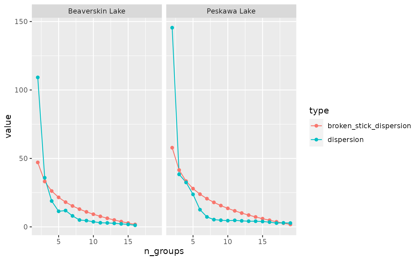
# plot broken stick dispersion to verify number of plausible groups
library(ggplot2)

nested_coniss %>%
  select(location, broken_stick) %>%
  unnest(broken_stick) %>%
  tidyr::gather(type, value, broken_stick_dispersion, dispersion) %>%
  ggplot(aes(x = n_groups, y = value, col = type)) +
  geom_line() +
  geom_point() +
  facet_wrap(vars(location))