Chapter 12 The Processing Toolbox

12.1 Purpose

Learn how to use the Processing Toolbox to maniuplate vector and raster data.

12.2 Tutorial

Open Minas Passage Raster, coastlines vector, profile vector
Create profile using the SAGA profile tool
Style Layers, use Print Composer to export
Optional exercise: contour Long Lake data using RST

Important note about using the processing toolbox: Some algorithms are sensitive to column names (particularly those in the GRASS toolbox). Words you are not allowed to have in your columns (upper case or lower case) can be found at this link. The most problematic of these is AS (as in, arsenic could be a column name). Spaces in your column names will also not go over well.

First, we will add the data required for the map. Using the Add Vector Layer dialog open the Browse file chooser.

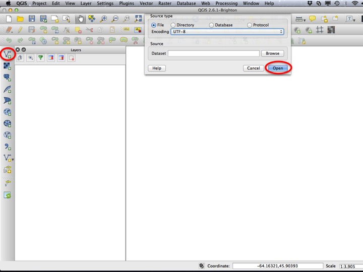
Slide01

Open the long_lake_depths and long_lake_outline layers from the “10 Interpolation Contouring” folder.

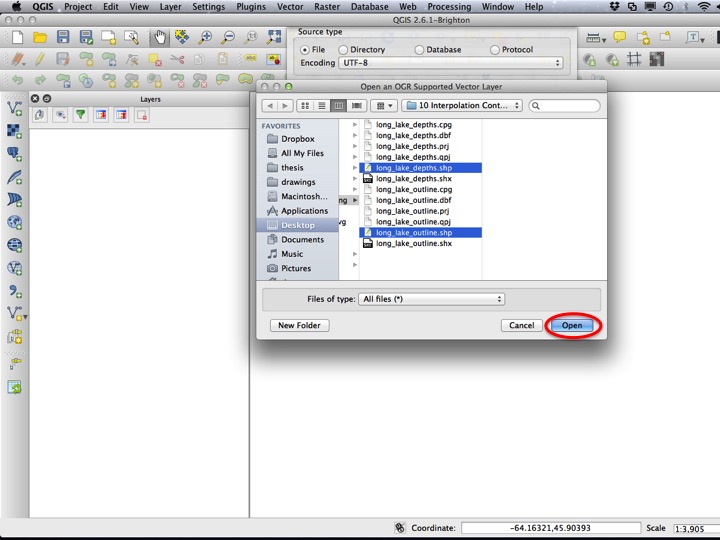
Slide02

12.2.1 The Processing Toolbox

You should make the water look like water, and it will help you verify your results later if you label your points. To open the Processing Toolbox, choose Toolbox from the Processing menu.

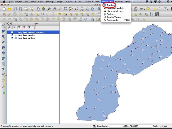
Slide03

This should open a panel that has a list of processing algorithms. If you don’t see “GRASS” in the list, tell the instructor! You will need to install the “GRASS” plugin using the Plugin Manager.

12.2.2 Interpolation

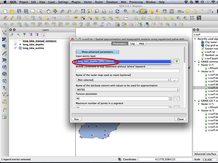
We will run one of these “geoalgorithms” to interpolate between the points to create a surface or raster layer that represents the same information. The algorithm we will use is called “v.surf.rst”, and is short for Regularized Spline Tension. Double click the name to bring up the algorithm window.

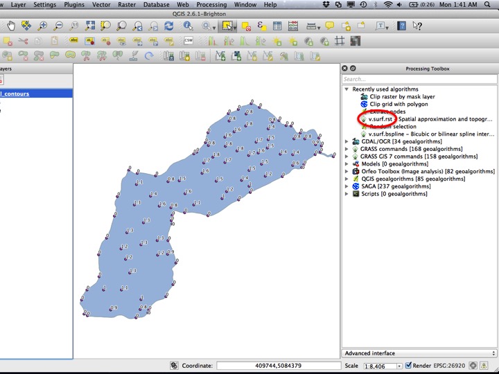
Slide04

In the algorithm window, choose the Input points layer as “long_lake_depths”.

Slide05

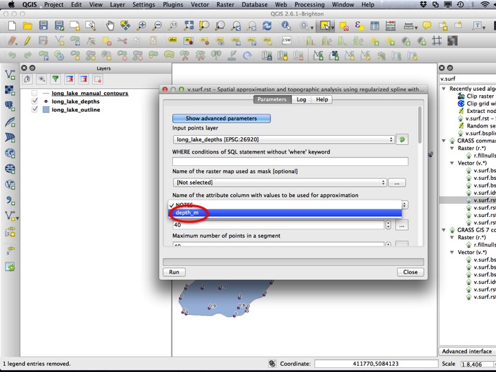
Next, we have to pick the attribute column that contains our “known” depth values. This is “depth_m”.

Slide06

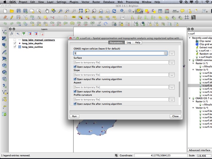
The other option we have to pick is the output cell size. Rasters are a collection of cells, and if this number is too small the file size will be huge, or if it is too big then the raster won’t have enough resolution to describe the surface. For now, set this value to 5 (metres). Click Run to run the algorithm.

Slide07

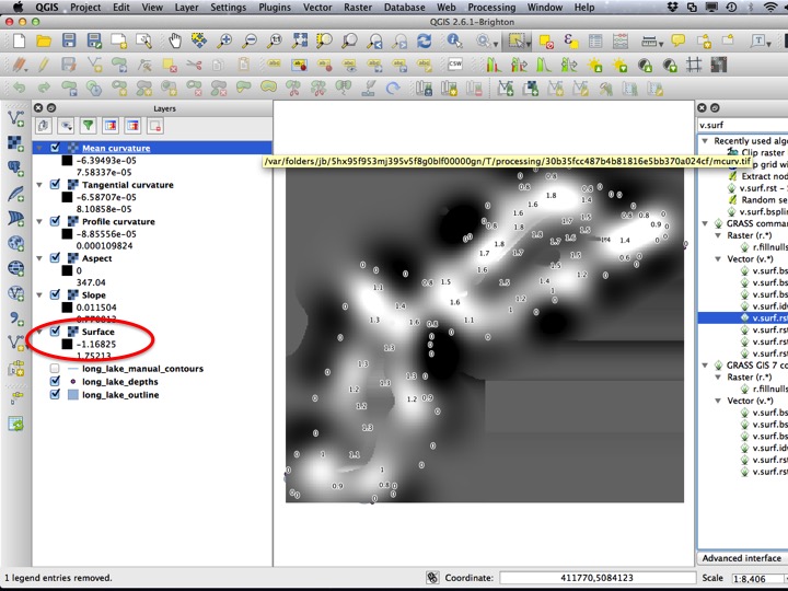
With any luck, you should see a bunch of layers pop up on your screen. Then one you are interested in is the one labeled “Surface”. Remove the other layers.

Slide08

Let’s inspect this raster using the Identify tool. Click near the labeled points to see if the raster approximated the known points correctly.

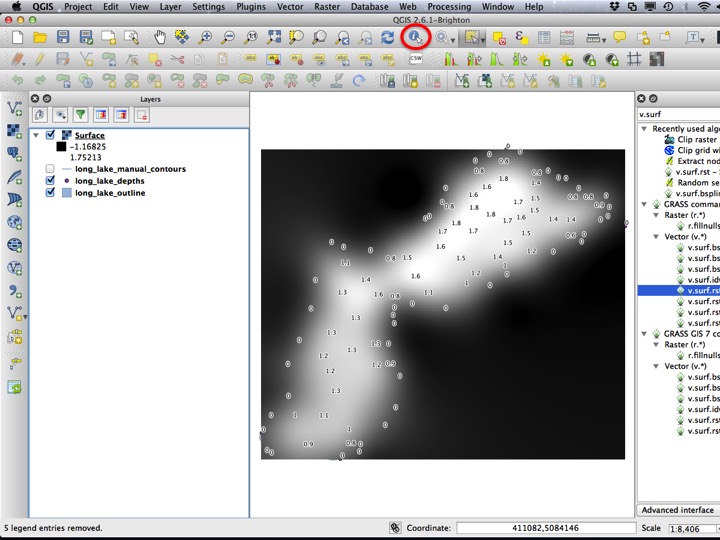
Slide09

In our case, we want to clip this surface to the edge of the lake, since it doesn’t apply outside the lake. We can do this using another algorithm called “Clip grid wih polygon”.

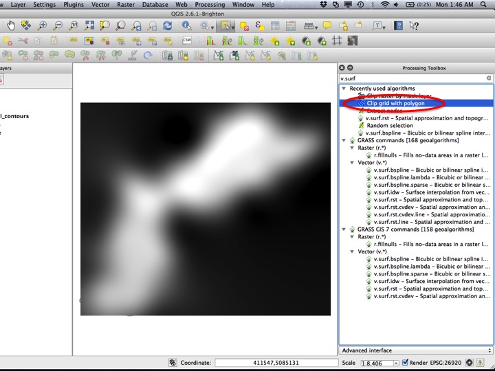
Slide10

The Input layer is “Surface”, and the Polygons layer is “long_lake_outline”. Choose Run to run the algorithm.

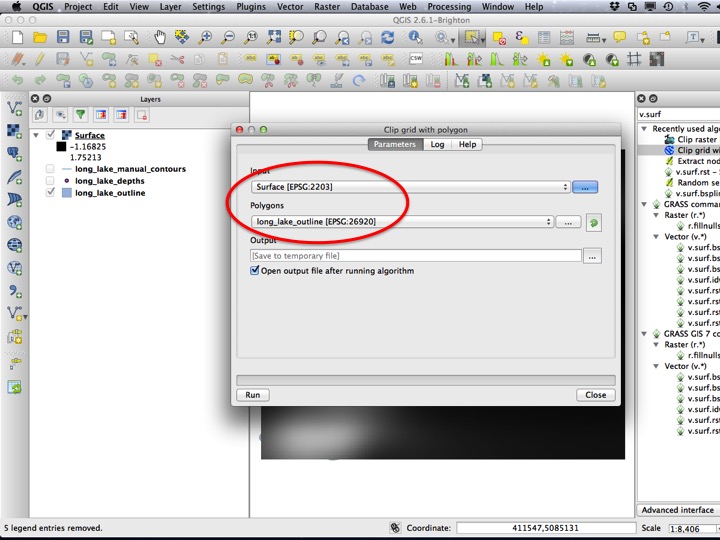
Slide11

It may try to tell you that the layers do not have the same CRS. In our case this isn’t true, but if you get this message in real life and get unexpected results, you should make sure the layers have the same CRS before trying again.

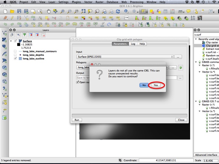
Slide12

The output should be a raster layer that only has values inside the lake boundary. Remove the “Surface” layer.

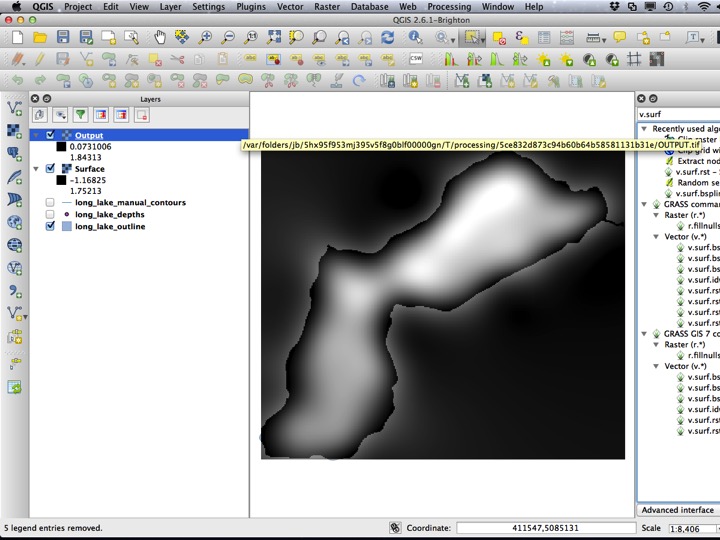
Slide13

12.2.3 Contouring

There is another geoalgorithm that will draw contour lines based on a raster surface. This algorithm is called “r.contour.step”.

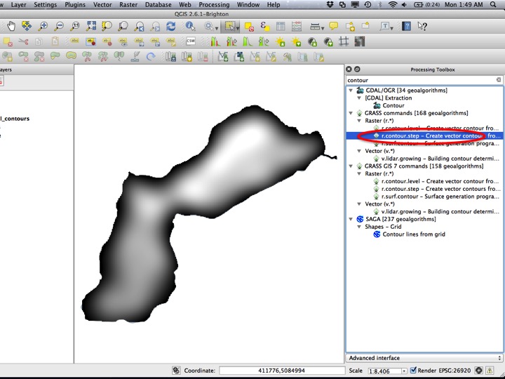
Slide14

Our Input raster is the “Output” layer, the minimum contour level is 0.5, the maximum is 2, and the interval is 0.5 m.

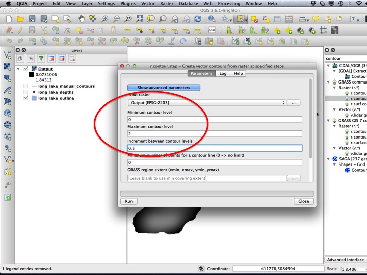
Slide15

When the algorithm is run, you should have a layer called “contours”. If you did your hand contouring well, the computer generated contours should look similar to your own.

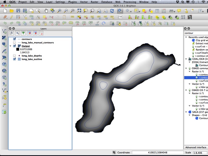
Slide16

12.2.4 Saving the files

So far, your files haven’t been saved! They are temporary files, which is great for trying a bunch of things, but not great if you close your project and forge to save them. Always save the outputs of your processing algorithms once you’ve decided to keep them. We will start by saving the raster layer “Output”.

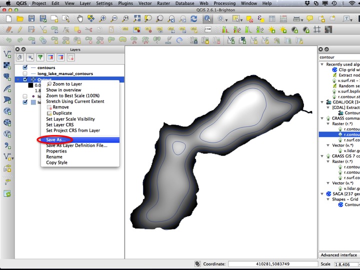
Slide17

Choose a location in which to save the raster output.

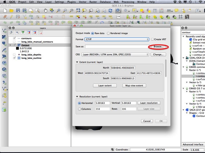
Slide18

Save it as something descriptive in the tutorial folder.

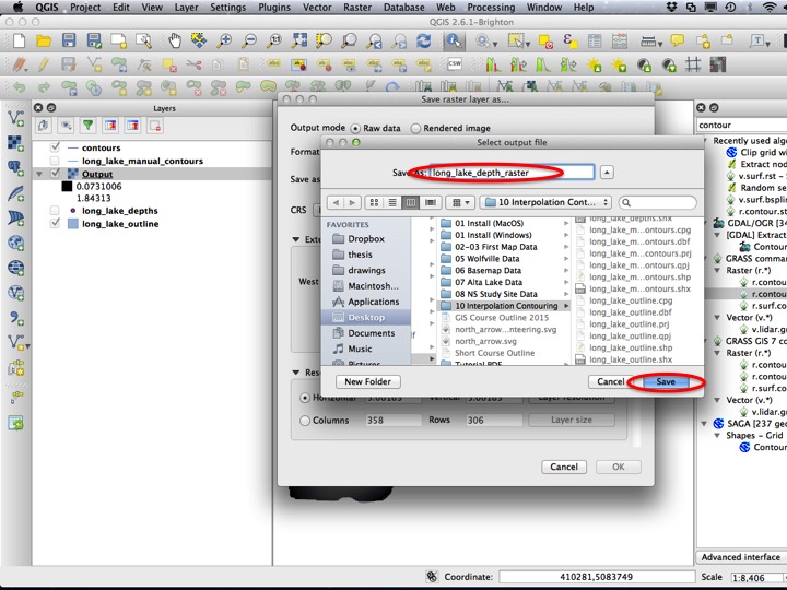
Slide19

Press OK to save the raster layer.

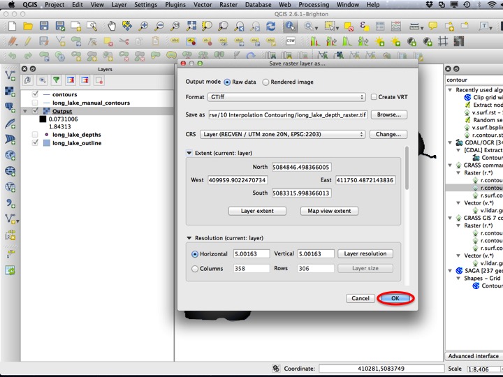
Slide20

Next we will save the “contours” layer. Right click and choose Save As….

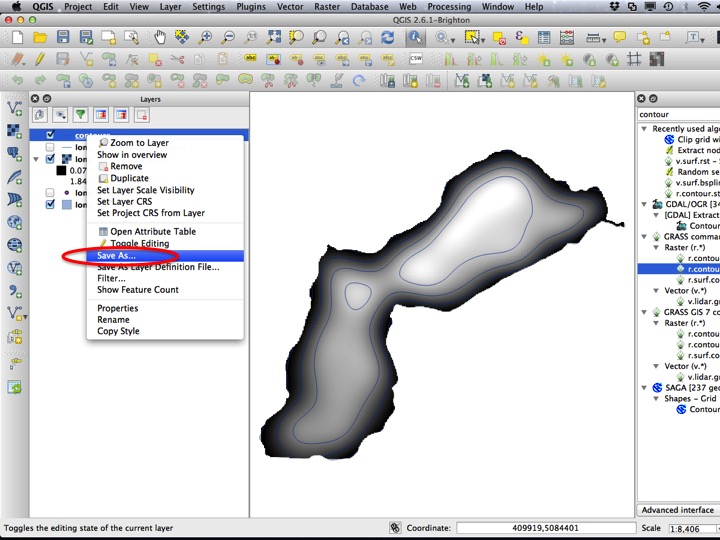
Slide22

I usually save contour layers with the contour interval somewhere in the name of the file.

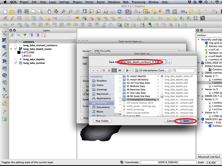
Slide23

Remove the temporary layers, and you should have a project that looks like this.

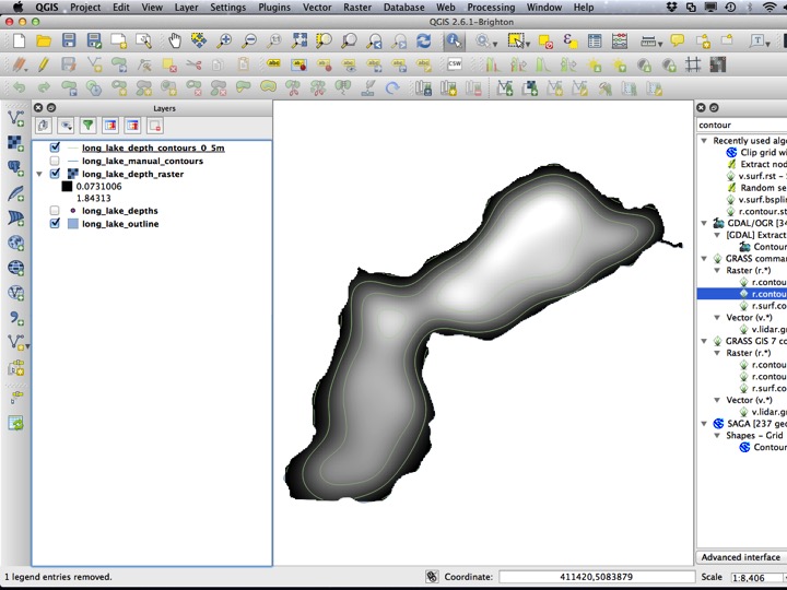
Slide24

12.2.5 The Assignment

For this module, use the Print Composer to create a PDF version of the map you have created. You can choose to include the raster layer or not, but if you do, you should include it in the legend. Your map should look something like the image below.

The Assignment