Tutorial 1 Basic R
When you open RStudio, you are presented with the ominous > of the R console. By the end of this tutorial, hopefully that > should fill you with a feeling of hope and opportunity, for magical things can happen when you type the right thing after the >. This short introduction will get you started with the R console so that when we introduce more powerful functions, you can understand what R is doing at the base level! The tutorial is loosely based on the Workflow: basics tutorial in the free online book, R for Data Science (Grolemund and Wickham 2017).
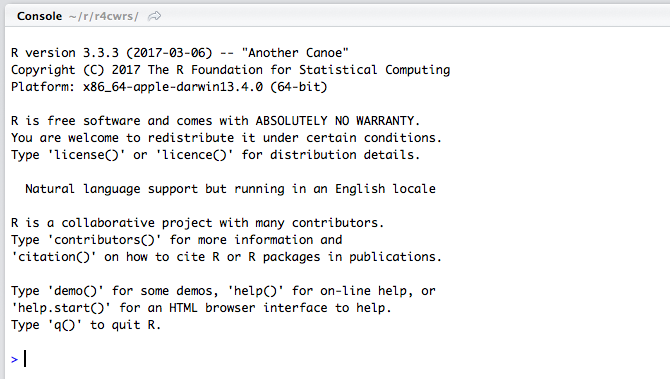
The basic R console.
1.1 Prerequisites
The prerequisite for this tutorial is the tidyverse package. If this package isn’t installed, you’ll have to install it using install.packages(), which you can type after the >.
Load the packages when you’re done! If there are errors, you may have not installed the above packages correctly!
## ── Attaching packages ────────────────────────────────── tidyverse 1.2.1 ──## ✔ ggplot2 2.2.1 ✔ purrr 0.2.4
## ✔ tibble 1.4.2 ✔ dplyr 0.7.4
## ✔ tidyr 0.8.0 ✔ stringr 1.3.0
## ✔ readr 1.1.1 ✔ forcats 0.3.0## ── Conflicts ───────────────────────────────────── tidyverse_conflicts() ──
## ✖ dplyr::filter() masks stats::filter()
## ✖ dplyr::lag() masks stats::lag()1.2 Expressions and Variables
Let’s start with the basics. Try typing in something like this at the prompt:
## [1] 2## [1] 10## [1] 25## [1] 12As you can see, R works just like a calculator and evaluates all of these expressions just like you would expect. If we would like to save the result of one of these expressions we can assign that value to a variable like this:
Then, to view the value of x we can just type x at the console, and R will show us the value.
## [1] 2The <- means “assign the value on the right to the variable on the left”. We can also use x in any expression and R will substitute its value in like this:
## [1] 4An expression is something that R can evaluate to produce a value, like 2+2 or x + 2. Any time you type this in the console without assigning it to a variable, R will print out the value. In fact, any time you type anything into the R console, R is evaluating that expression, which may or may not return a value. If there is no value returned, R won’t print anything when you press enter.
So far we’ve just used numbers, but often we need to enter text into R. Whenever we do this, we surround the text in quotes, like this:
Text (called character vectors) are one of many data types available in R.
1.3 Functions
A function is some kind of operation that takes one or more arguments (input values) and produces a return value (output value). The sqrt() function is a good example:
## [1] 2Here, 4 is an argument, and the function returns the square root of that, which is 2. Functions can take more arguments, like the max function:
## [1] 10Here we are giving the max function 5 arguments, of which it returns the maximum. One other way we specify arguments is by keyword arguments, like in the paste function.
## [1] "string1_string2"The paste function takes its arguments and combines them using the sep that we specify, in this case "_". The function returns this string. Many functions in R have many many arguments and usually we only want to modify one or two of interest to us. The format is always key=value, where key is the name of the keyword and value is some expression we would like to use as the value for that argument.
R contains thousands of functions that do most of what you could possibly imagine with regards to data and statistics, but remembering which one you want and how to use it can be difficult. Luckily, RStudio makes it easy using tab autocompletion and easy access to help files. To autocomplete, start typing the name of the function and press the [Tab] key (or Ctrl+Space), and RStudio will helpfully provide you with suggestions.
To access the documentation for a particular function, you can type ? in front of the function name and press return, and RStudio will open the help file for you if it exists.
Will bring up the following:
1.3 Description
Concatenate vectors after converting to character.
1.3 Usage
paste (..., sep = " ", collapse = NULL)
paste0(..., collapse = NULL)
1.3 Arguments
…one or more R objects, to be converted to character vectors.
sepa character string to separate the terms. Not
NA_character_.collapsean optional character string to separate the results. Not
NA_character_.
Note that each of these arguments can be specified by keyword, and have default values that we can see in the usage section. The ... means that we can pass any number of arguments to the function. There’s too many functions in R to keep in your head at one time, so getting good at reading these help files is very useful!
1.4 Vectors
So far we’ve just been dealing with single values like 2+2 or "mystring", but the real power of R is that it can operate easily on large lists of data, so it makes sense that it provides us with an easy way to work with this data. These lists of data are called vectors, and we create them using the c function (c stands for concatenate, or join together).
## [1] 10 9 8 7 2Here the c function took our arguments of 10, 9, 8, 7, and 2, and returned a vector, which we assigned to the variable named myvector. When we evaluated myvector, it printed out the list of values it contained.
Vectors don’t just have to contain numbers, they can contain strings as well.
## [1] "word1" "word2" "word3"Here the c function took our arguments and returned a vector of strings, which we assigned to the variable mytextvector.
It is common to have to generate a vector of all the integer values between two numbers, so R provides a short form for this:
## [1] 1 2 3 4 5 6 7 8 9 10## [1] 20 19 18 17 16 15 14 13 12## [1] 13 14 15 16You can also use an expression on either side of the :, like this:
## [1] 25 26 27 28 29 30## [1] 25 26 27 28 29 301.5 Indexing
Now we’ve created vectors, but to get at what’s inside them we need to retrieve values using an index. We do this using square brackets like this:
## [1] 10## [1] 2## [1] 8This code creates a vector, assigns it to the variable myvector, then retrieves the 1st, 5th, and 3rd value stored in that vector. If we would like multiple values from the vector, we can pass multiple values as indices, like this:
## [1] 10 2 8You’ll notice that the index that we’re using is actually a vector itself! I know, we’re using a vector to index a vector and it’s a little trippy, but it’s incredibly useful. You’ll remember that we can easily create vectors of sequential integers, which we can use to get a sequence of values from a vector by using it as an index.
## [1] 10 9 8This would be equivalent to:
## [1] 10 9 8There is one other useful way to index a vector using a vector, which is to use a TRUE/FALSE vector. This is probably the most useful of the indexing methods, because it allows you to do things like:
## [1] 10 9 8This works because myvector > 7 is, itself, a TRUE/FALSE vector with the same length as myvector, indicating whether or not it is greater than 7 at any given position.
## [1] TRUE TRUE TRUE FALSE FALSE1.6 Missing Values
Missing values are represented in R using NA, or “not assigned”. The fact that R handles missing values is one of the best reasons to use R for data analysis, because missing values are common in real data. NA values are propogated by R functions, meaning that if you take the mean() of a vector containing a missing value, it will give you NA as the average!
## [1] NAThis is rarely what you want, but is a good practice to explicitly handle missing values in your code, and R forces you to do this. To avoid getting an NA back, you can use na.rm = TRUE, an argument that is available in many R functions.
## [1] 21.7 Data Frames
The vast majority of data in R is kept in a tibble (often called a data frame), which is a collection of vectors of the same length. You can think of a tibble as a table, with each column in the table being of the same type (numeric, character, TRUE/FALSE, etc.).
my_tibble <- tibble(
  number = c(1, 2, 3),
  name = c("one", "two", "three"),
  is_one = c(TRUE, FALSE, FALSE)
)
my_tibble
## # A tibble: 3 x 3
## number name is_one
## <dbl> <chr> <lgl>
## 1 1 one TRUE
## 2 2 two FALSE
## 3 3 three FALSEThe syntax for creating a tibble is tibble(column_name = value). The above tibble has three columns (number, a numeric column, name, a character column, and is_one, a logical TRUE/FALSE column). You can get these values as vectors again using the $ operator, which allows you to extract a vector from a data frame.
## [1] 1 2 3## [1] "one" "two" "three"## [1] TRUE FALSE FALSEYou can think of tibbles as a collection of vectors (variables) having the same number of elements. The number of elements has to be equal for all columns, meaning the ith value of each vector forms an observation. Data in this form is very useful and is the subject of most of the following tutorials.
1.8 Loading Packages
Basic R functionality is designed to provide basic functions to help with data analysis, but may add-ons are available and code you find online (including here, shortly) will often tell you to load a “package” using library(). This will be a call to the library() function in the form library(packagename), where packagename is the name of the package which contains the functions you are interested in using (all of the subsequent tutorials will use library(tidyverse), because the tidyverse package contains many useful functions that you will use on a regular basis. When you call library(packagename), it will make these functions available to you. Occasionally you will see something like packagename::function_name(), which is a method to use a function without making all of the functions in a package. This is equivalent to typing library(packagename) then function_name() on the next line. You can install packages using install.packages("packagename") (note the quotes around packagename!).
For example, let’s install the tidyverse package now, since you’ll be using it in the rest of this series.
Then, load it using library():
Finally, we are ready to call a function from the package. The tidyverse package actually installs and loads a family of useful packages for us, a list of which we can access using tidyverse_packages(). Try it!
##  [1] "broom"       "cli"         "crayon"      "dplyr"       "dbplyr"
##  [6] "forcats"     "ggplot2"     "haven"       "hms"         "httr"
## [11] "jsonlite"    "lubridate"   "magrittr"    "modelr"      "purrr"
## [16] "readr"       "readxl\n(>=" "reprex"      "rlang"       "rstudioapi"
## [21] "rvest"       "stringr"     "tibble"      "tidyr"       "xml2"
## [26] "tidyverse"
1.9 Using the Script Editor
In reality, very little of the code you type will be directly in the prompt. Instead, you will use RStudio’s script editor to run commands so that you can go back and edit them or run them from the beginning. To create a new R script, choose File, New File, and R script (you can also choose the little green “+” button at the top left of the console window). A blank R script should appear in a new tab.
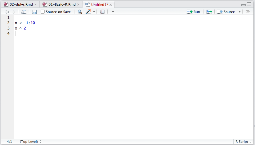
A new R script in the RStudio script editor.
When you type a command in the editor and press enter, nothing happens! This is because the editor is meant to build script that contain multiple lines, unlike the console, which is meant to execute a single line at a time. To run a command you have typed in the script editor, press Ctrl+Enter (Command+Enter on a Mac). You can even select multiple lines, press Ctrl+Enter, and they will all run at once! You can also save the script and choose Source to run the whole thing. It is good practice to keep all of your code in a script somewhere. Typing it on a console repeatedly is hard work, and leads to errors!
1.10 The Environment
When you’ve assigned a bunch of variables, it can be tricky to keep track of which ones are where and contain what! Hopefully you have given them short but descriptive names, but if you happen to forget you can check the “Environment” tab in RStudio (in the upper right part of the window). If you’d like to start fresh you can clear the environment (use the little broom icon or go to Session/Clear Workspace), and if you really want to start fresh, you can restart R using Session/Restart R. This will clear your workspace and unload all the packages you loaded using library(). This is a good way to make sure all of your analysis has been encapsulated by the script, since you can Restart R and Source your script to replicate your work.
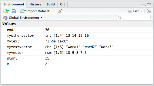
The RStudio Environment Tab
By default, R will save your session when you quit and reload the variables you had previously assigned when you reopen it. This is dangerous, because even though you created an object, you may not be able to create it again! I highly reccomend using the script editor to encapsulate all of your code, and disable the automatic loading/saving of your workspace. You can do this in RStuio’s Preferences (or “Global Options” on Windows/Linux) by setting “Save workspace on exit” to “Never”, and unchecking “Restore .RData into workspace at startup”.
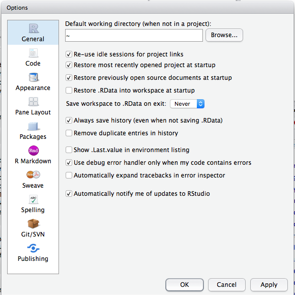
The RStudio Global Options/Preferences window.
1.11 Excercises
To practice the basics of R, complete the very first swirl module, R Programming / Basic Building Blocks. To do this, you’ll need to install and load swirl by typing this at the R prompt:
You should get a friendly greeting that will prompt you to choose a course (you want number 1, “R Programming: The basics of programming in R”) and a module (you want number 1, “Basic Building Blocks”). I suggest stopping after the first module, as R for Data Science provides a more effective introduction to the language.
1.12 Summary
In this lesson we covered expressions, variables, functions, vectors, and indexing, all of which will help you get the most out of the tutorials in this series. For more information, check out the Workflow: basics and Workflow: scripts tutorial in the free online book, R for Data Science.
References
Grolemund, Garrett, and Hadley Wickham. 2017. R for Data Science. New York: O’Reily. http://r4ds.had.co.nz/.