Chapter 16 Earth-System Change
Adapted from Physical Geology, First University of Saskatchewan Edition (Karla Panchuk) and Physical Geology (Steven Earle)
. Click the image for more attributions._](figures/16-earth-system-change/figure-16-1.png)
Figure 16.1: Antarctic Peninsula. Antarctica was not always covered by ice. A change in the Earth system triggered the onset of Antarctic glaciation approximately 40 million years ago. Source: Karla Panchuk (2018) CC BY-SA 4.0. Photo: Liam Quinn (2011) view source. Click the image for more attributions.
Learning Objectives
After reading this chapter, completing the exercises within it, and answering the questions at the end, you should be able to:
- Explain why it is useful to think of Earth as a system.
- Describe the effect of feedbacks on the climate system.
- Explain the difference between weather and climate.
- Describe the climate-forcing mechanisms related to insolation, heat transport over Earth’s surface, and changes in the atmosphere’s energy budget.
- Explain the difference between direct and proxy data about Earth’s climate, and give examples of each.
- Describe the role of computer models for understanding the Earth system.
- Summarize the history of human influence on the Earth system.
- Explain how carbon isotopes link rising atmospheric CO2 levels to fossil fuels burned by humans.
- Describe how humans have affected the present-day carbon cycle and why the human contribution is significant.
- Summarize the kinds of observations that show signals of present-day climate change.
- Describe the current and projected state of the Earth system in the Anthropocene Epoch.
16.0.0.1 The Only Constant Is Change
If one thing has been constant about the Earth system over geological time, it is unceasing change. In the geological record of climate, sedimentary deposits provide evidence of glaciations in the distant past; the chemical characteristics of sea-floor sediments tell about periods of extreme warmth. The Earth-system, and thus Earth’s climate, has not only changed frequently, but also with large temperature fluctuations. Today’s mean global temperature is approximately 16°C. During Snowball Earth episodes more than 600 million years ago, when Earth’s surface was frozen from pole to pole (or nearly so), the global mean was as cold as -50°C. At various other times in Earth history, it has been close to 30°C.
Part of this chapter addresses natural processes of climate change, how they work, and how we know what Earth’s past climate was like. Geologists study those natural climate-change processes to understand how human-caused, or anthropogenic, changes to the Earth system might affect the climate in the future, and how much the climate has changed over the time that humans increased their influence on the Earth-system. The rest of the chapter addresses what has been learned by asking those questions.
16.1 What Is the Earth System?
Earth can be characterized in terms of its “spheres.” The atmosphere is the envelope of gas surrounding the planet. The hydrosphere is the water on the planet, whether in oceans, rivers, glaciers, or the ground. The __biosphere __comprises living organisms. The __lithosphere __is the rocky outer shell of the planet.
Components of these spheres interact constantly, with processes occurring in one sphere having an impact in other spheres. Cycles such as the water cycle or the carbon cycle constantly move matter and energy between spheres. Taking an Earth-system approach—looking at how the spheres are connected—is a way to account for the web of interactions responsible for the “big picture” of the Earth that we know.
The climate change related to the opening of the Drake Passage (Figure 16.2) is a good example of why a system of interactions is needed to understand how Earth works. The Drake Passage (bottom left map) is the gap between the southern-most tip of South America, and Antarctica.
Prior to 40 million years ago, the Drake Passage did not exist (top left map), and neither did the Antarctic ice cap. The arm of land connecting South America and Antarctica allowed warm ocean currents (red arrows) to carry heat from the equator to Antarctica. When the gap opened up, a new cold-water current formed (blue arrows) that blocked warm water from reaching Antarctica. Without the warm current, Antarctica froze over.
). Click the image for more attributions and terms of use.](figures/16-earth-system-change/figure-16-2.png)
Figure 16.2: An example of Earth-system interactions. The opening of the Drake Passage changed how ocean currents moved heat around the planet, and cooled Antarctica until it froze over. Source: Karla Panchuk (2018) CC BY-NC-SA 4.0. Map: Modified after Woods Hole Oceanographic Institution (view source). Click the image for more attributions and terms of use.
There were many interconnecting processes within the Earth-system (Figure 16.2, right) that drove glaciation in Antarctica. First, heat energy within Earth drove plate tectonics (lithosphere), making it possible for South America to separate from Antarctica. This impacted ocean currents (hydrosphere), and ultimately how water was stored on Antarctica (hydrosphere) by changing the climate of Antarctica.
In the Earth system, nothing happens in isolation. The change in the climate of Antarctica had a global impact. The ice cap on Antarctica increased Earth’s albedo, the reflectiveness of Earth’s surface. The more reflective Earth’s surface, the more of the sun’s light is reflected back into space without heating Earth. This caused even more ice to form, and cooled the planet as a whole.
When Earth cools, the change in temperature has a cascade of effects including changing precipitation patterns (hydrosphere), and changing the characteristics of habitats (biosphere). When habitats cool, organisms needing more warmth will migrate closer to the equator. This is true of plants as well as other forms of life.
Ice is not the only type of land cover that affects albedo—forests do as well. Forests also increase local atmospheric moisture levels through transpiration, when they release water vapour into the atmosphere. Local temperature and moisture differences also affect rainfall patterns on top of larger-scale changes resulting from cooling.
The chain of events in summarized in Figure 16.2 is only a broad overview of all of the consequences of opening a gap between South America and Antarctica. For example, it does not include the effects of what a change in the types of plants in a location does to local weathering and erosion. Trees can accelerate weathering, releasing more nutrients from rocks into runoff, which can affect algae blooms in water bodies, which in turn reduces oxygen levels in the water, which affects organisms living in the water that rely on oxygen.
Trees growing along a river can also slow the rate of erosion, reducing the amount of sediment in the river, and ultimately the rate of development of a delta at the river’s mouth. Deltas undergo subsidence as accumulated sediments are compressed, so if the sediment supply is reduced, parts of the delta may become flooded, changing the extent of wetlands. Wetlands with waters depleted in oxygen can prevent plant material from decaying and releasing their carbon back into the carbon cycle as carbon dioxide. Changing atmospheric carbon dioxide levels alters the way energy moves through Earth’s atmosphere, and affects Earth’s surface temperatures.
The short version of why it’s important to look at Earth as a system is that everything is connected, so that a change in one part of the system can ripple through the rest of the system and have effects well beyond any one location or time.
16.1.1 Feedbacks Amplify or Diminish Earth-System Change
The web of interactions in the Earth system is complex, but there is yet another level of complication. Sometimes a change in the Earth system can trigger other changes that have the effect of amplifying the original change, or diminishing it. The series of interactions that amplify or diminish a change are called feedbacks. A feedback that amplifies change is called a positive feedback. A feedback that diminishes the size of a change is called a negative feedback.
In the events related to the glaciation of Antarctica, the formation of ice is an example of a positive feedback. Ice formation was caused by cooling, but it triggered even more cooling by reflecting sunlight away from Earth’s surface. This is called ice albedo feedback. An example of a negative feedback is plant growth. Plants need CO2 to make food, so as long as the plants have enough nutrients and water, and temperatures are still suitable, increasing CO2 in the atmosphere could increase plant growth. Plant growth would draw down atmospheric CO2, so that there would be less warming than would otherwise be expected from the initial rise in atmospheric CO2 levels.
16.1.1.1 Misconceptions About Feedbacks
There are two common misconceptions about feedbacks. One misconception is that positive feedbacks result in changes that are good, and negative feedbacks result in changes that are bad. In fact, whether a feedback is positive or negative is unrelated to whether or not the change would be considered a good thing. For example, if a feedback accelerates warming and makes an ecosystems uninhabitable for animals that used to live there, it would still be a positive feedback even though it had a negative impact on the animals in that ecosystem. A feedback that slowed the rate of warming and gave the animals time to adapt would still be considered a negative feedback even though it helped the animals to survive.
Another misconception is that a positive feedback always results in some value increasing (e.g., a rise in temperature), and a negative feedback results in a decrease in that value. Positive feedbacks can cause a value to decrease (e.g., as ice forms more sunlight is reflected, leading to decreased temperatures), and negative feedbacks can cause a value to increase. What matters is whether the initial change is amplified or reduced, not which way the numbers are changing.
16.1.2 Feedbacks and Instability in the Earth System
The potential for sudden extreme changes in the Earth system depends on what feedbacks are available. At times when Earth’s climate was much warmer than today, no glaciers were present. When the climate is much cooler, a relatively small decrease in temperature could be enough to start the formation of ice and trigger the ice albedo feedback. However, if the climate is much warmer, the same decrease in temperature would not cool Earth enough to trigger the ice albedo feedback, and further climate cooling would be avoided. The reverse is also true- if warming occurs in a climate that is cold enough for glaciers to form, some of that ice might melt, reducing the albedo of Earth’s surface, and permitting even more warming. On the other hand, if the climate is already too warm for ice to exist, a small amount of warming won’t be amplified in the same way.
The albedo effect is not the only feedback that can make cooler climates less stable. Melting of permafrost (sediment that remains frozen year round) can also have an impact. Frozen soil contains trapped organic matter that is converted by micro-organisms to CO2 and methane (CH4) when the soil thaws. Both these gases contribute to warming when they accumulate in the atmosphere. Additional warming can cause even more permafrost to melt, permitting even more activity by micro-organisms, and releasing more CO2 and CH4.
Either of these feedbacks is enough on their own to accelerate climate change, but when they are both present together, the effect is even stronger. What this means is that the conditions in the Earth system before a change happens—called the initial conditions—play an important role in determining the impact of any changes that occur. A change that would have little impact under one set of initial conditions could have far reaching effects under another. Thinking of Earth as a system is a way to factor in the initial conditions. Otherwise we would be very puzzled why a small rise in global temperatures at one time in Earth history could have almost no discernible effect, but the same rise in temperatures at another time could lead to profound change.
16.2 Causes of Climate Change
16.2.1 What Is Climate?
Our day-to-day experience of the Earth system is in the form of the conditions we experience at Earth’s surface. The daily conditions that we think of as weather—the temperature, presence or absence of precipitation, winds, humidity, and so on—are a snapshot of the state of the Earth system at a particular instant in time and in a particular location. The weather that we get is variable, but in Saskatchewan most people would not be surprised to experience summer days with temperatures of 20 °C to 30 °C, and winter days with temperatures between –20 °C to –30 °C. Our notion of what summers and winters are generally like reflects our understanding of Saskatchewan’s climate. If we get a day in July with a daytime high of 10 °C, that would seem like unusually cold weather because we know it is uncharacteristic of the climate over all.
We characterize the climate by collecting data about the weather every day, and then calculating the average conditions over a period of decades. The Government of Canada provides averages for the periods 1961 to 1990, 1971 to 2000, and 1981 to 2010 in an online database that is searchable by geographic location or station. Data measured at Saskatoon’s Diefenbaker International Airport show that the average annual temperature from 1981 to 2010 is 0.6 °C higher than the annual average from 1961 to 1990, due warmer conditions in the winter and early spring (Figure 16.3).
. [View YXE data for 1981 to 2010](http://climate.weather.gc.ca/climate_normals/results_1981_2010_e.html?searchType=stnName&txtStationName=saskatoon&searchMethod=contains&txtCentralLatMin=0&txtCentralLatSec=0&txtCentralLongMin=0&txtCentralLongSec=0&stnID=3328&dispBack=0)._](figures/16-earth-system-change/figure-16-3.png)
Figure 16.3: Average temperatures for the periods 1961 to 1990, and 1981 to 2010 measured at Saskatoon’s Diefenbaker International Airport (YXE). Source: Karla Panchuk (2018) CC BY 4.0. View YXE data for 1961 to 1990. View YXE data for 1981 to 2010.
The climate as represented by the 1961 to 1990 interval was slightly cooler than the climate represented by the 1981 to 2010 interval. People who lived in Saskatoon between 1961 and 2010 may or may not have a sense that the weather they experienced from day to day was different for those intervals. In fact, some may have the record high of 35.3 °C on September 4, 1978 seared into their memory, and feel that Septembers just aren’t as hot as they used to be. They would be correct that as of 2017, there are no September temperatures recorded at the Diefenbaker International Airport weather station with a daytime high greater than 35.3 °C. But if that gave them the impression that Septembers are cooler on average today than in the past, that would not be consistent with the data.
16.2.2 Climate-Forcing Mechanisms
A climate-forcing mechanism is a process that causes climate to change. Climate forcings work by initiating changes in how heat energy moves into, through, and out of the Earth system. When we discuss a particular climate change event, the climate-forcing mechanism is what initiated the change. Feedbacks also alter climate, but we want to know what triggered the feedbacks in the first place.
16.2.2.1 Climate Forcing by Changes in Insolation
Insolation, or incoming solar radiation, refers to how much of the sun’s energy reaches Earth’s surface in a given period of time. Insolation is measured in Watts per square meter (W/m2).
16.2.2.1.1 Long-term Solar Evolution
Over the long term (billions of years), stars like our sun become larger, brighter, and hotter (Figure 16.4). Earth receives 40% more heat from the sun today than it did 4.5 billion years ago. In Figure 16.4, the blue _Now _arrow shows the sun’s current point in its life history. Although the blue arrow appears to indicate an instant in time, the time interval reflecting the duration of human existence on Earth is but a tiny fraction of the width of the line. As far as human experience is concerned, the long-term evolution of the sun is so slow that it has made no difference at all on insolation for the entire time humans have existed.
_](figures/16-earth-system-change/figure-16-4.png)
Figure 16.4: The life history of a star, from condensation of a nebula, to expansion to a red giant, and ending as a white dwarf. Source: Karla Panchuk (2017) CC BY 4.0. Modified after Oliver Beatson (2009) Public Domain view source
16.2.2.1.2 Orbital Cycles
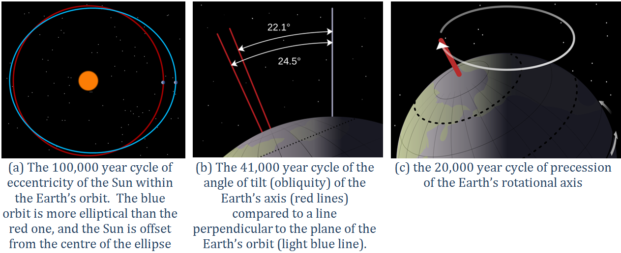
Insolation is also affected by cyclical changes in Earth’s orbit and rotation. Over intervals of approximately 100,000 years, the __eccentricity __of Earth’s orbit changes. Eccentricity is a measure of how elliptical a circle is. Higher eccentricity means that the orbit is more elliptical (Figure 16.5, left, blue orbit), whereas lower eccentricity means the orbit is more circular (Figure 16.5, left, red orbit). Eccentricity is important because when it is high, the Earth-sun distance varies more from season to season than it does when eccentricity is low.
. Click the image for more attributions._](figures/16-earth-system-change/figure-16-5.png)
Figure 16.5: Cycles in Earth’s orbit. Left: The shape of Earth’s orbit (its eccentricity) changes over 100,000 year cycles from more circular to more elliptical. Middle: Over 41,000 year periods, Earth’s axis of rotation nods toward and away from the sun. Right: Over 21,000 year cycles, Earth wobbles on its axis of rotation. Source: Karla Panchuk (2017) CC BY 4.0. Modified after Steven Earle (2015) CC BY 4.0 view source. Click the image for more attributions.
Over intervals of approximately 41,000 years, the __obliquity __of Earth’s axis of rotation changes (Figure 16.5, middle). This results in a nodding motion that alters how directly the sun shines on Earth’s poles. When the angle is at its maximum (24.5°), Earth’s seasonal differences are accentuated. When the angle is at its minimum (22.1°), seasonal differences are minimized.
Cycles of __precession __happen over intervals of approximately 20,000 years, causing Earth’s axis of rotation to wobble (Figure 16.5, right). This means that although the North Pole is presently pointing to the star Polaris (the pole star), in 10,000 years it will point to the star Vega.
The importance of eccentricity, tilt, and precession to Earth’s climate cycles (now known as Milanković Cycles) was first pointed out by Yugoslavian engineer and mathematician Milutin Milanković in the early 1900s. Milanković recognized that although the variations in the orbital cycles did not affect the total amount of insolation that Earth received, it did affect where on Earth that energy was strongest. Glaciations are most sensitive to the insolation received at latitudes of approximately 65°. As continents are configured today, this is most significant at 65° N, because there is almost no land at 65° S.
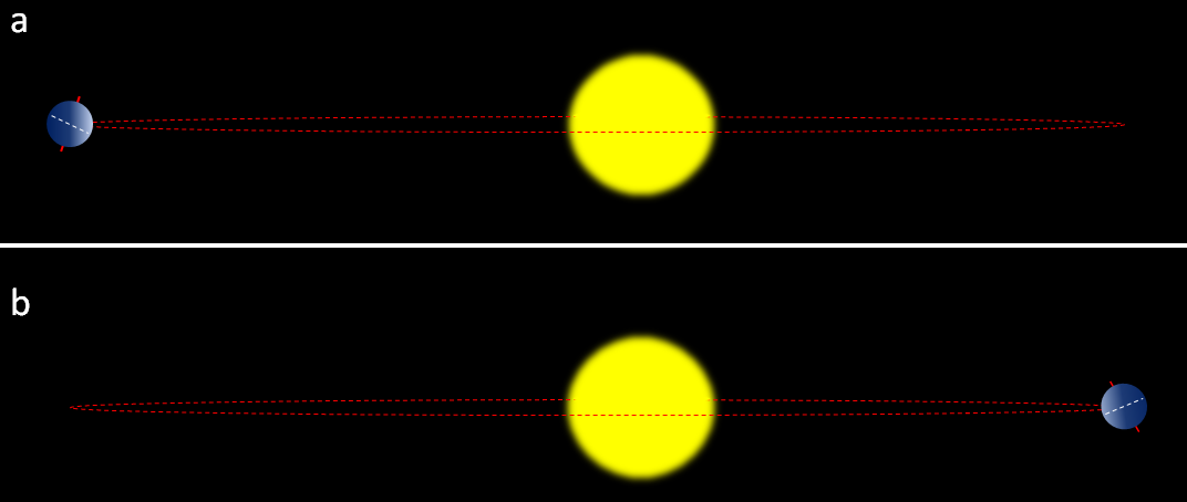
The most important factors are whether the northern hemisphere is pointing toward or away from the sun at its closest or farthest approach, and how eccentric the sun’s position is in Earth’s orbit. For example, if the northern hemisphere is at it farthest distance from the sun during summer (Figure 16.6, top), this means cooler summers. If the northern hemisphere is at its closest distance to the sun during summer (Figure 16.6, bottom), this means hotter summers. Cool summers — as opposed to cold winters — are the key factor in the accumulation of glacial ice, so the upper scenario in Figure 16.6 is the one that promotes glaciation. This factor is greatest when eccentricity is high.
_](figures/16-earth-system-change/figure-16-6.png)
Figure 16.6: Effect of precession on insolation in the northern hemisphere summers. In (a) the northern hemisphere summer takes place at greatest Earth-sun distance, so summers are cooler. In (b) (10,000 years or one-half precession cycle later) the opposite is the case, so summers are hotter. The red dashed line represents Earth’s path around the Sun. Source: Steven Earle (2015) CC BY 4.0 view source
The effects of all three cycles are evident in geochemical climate data. Figure 16.7 shows the “signals” for obliquity (A), eccentricity (B), and precession (C) over a period from 800,000 years in the past, to 800,000 years in the future. The vertical black line running down the middle of the diagram marks the present day. When the insolation from all three signals is determined, the result is a more complex waveform (D) with times of low variation in insolation, and times with higher variation in insolation.
 Click the image for more attributions._](figures/16-earth-system-change/figure-16-7.png)
Figure 16.7: Comparison of orbital cycles, insolation, and climate data for a 1.6 million year period. Source: Karla Panchuk (2017) CC BY-SA 4.0, modified after Incredio (2009) CC BY 3.0 view source. Click the image for more attributions.
The graphs E and F are climate information measured in microfossils dwelling at the ocean floor (E) and in water from ice cores (F). Peaks in temperature in F correspond to peaks in the oxygen isotope record in E, which indicate that it was warmer, there was less ice, and sea level was higher. Troughs are times when Earth was deep within an ice age. It was cooler, there was ice on land, and sea level was lower.
The vertical dashed lines on the left-hand side of Figure 16.7 mark the times of peak warm temperatures and allow for comparison of the timing of the temperature peaks with the timing of the orbital cycles. Peak temperature events are approximately 100,000 years apart, suggesting that the eccentricity cycle might be the most important contributor. Indeed, in B most (but not all) of the peak temperature events correspond to a time when Earth’s orbit was at or near peak eccentricity for that cycle.
It is tempting to conclude that eccentricity is the most important orbital cycle for climate change over all. However, this pattern only began a little over 1 million years ago. For 1.5 million years before that, the 41,000-year obliquity cycle seems to dominate insolation cycles.
In general, times of warmest or coolest temperatures don’t line up perfectly with orbital cycles. There is no one orbital cycle that is most important for all of Earth history. It is also the case that changes in insolation due to orbital cycles are not sufficient to cause temperatures to change as much as the geological record says they have; feedbacks must be factored in to explain the observed temperature changes.
16.2.2.1.3 Sunspot Cycles
Sunspots are dark patches that appear on the surface of the sun as a result of intense local disturbances in the sun’s magnetic field (Figure 16.8, left). Loops of plasma (gas with electrical charge, Figure 16.8, right) follow along magnetic field lines from one sunspot to another.
. Right- NASA/Solar Dynamics Observatory (2015) Public Domain [view source](https://www.nasa.gov/content/coronal-loops-in-an-active-region-of-the-sun)._](figures/16-earth-system-change/figure-16-8.png)
Figure 16.8: Sunspots. Left: Photograph of sunspots with dots representing the size of Earth and Jupiter for scale. Right: Plasma loops viewed in x-ray wavelengths jumping from one sunspot to another on the sun’s surface. Source: Left- NASA/Solar Dynamics Observatory (2012) Public Domain view source. Right- NASA/Solar Dynamics Observatory (2015) Public Domain view source.
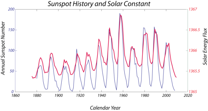
Sunspots appear dark because they are lower-temperature regions on the sun’s surface. For that reason you might think that more sunspots means a reduction in insolation. In fact, just the opposite is true, because sunspots are a side-effect of increased solar activity. Peaks in the number of sunspots counted annually since approximately 1870 (Figure 16.9, blue), coincide with peaks in measurements of solar energy output from the same time period (Figure 16.9, pink).
. Global average temperature modified after Met Office (2015) Contains public sector information licensed under the [Open Government Licence v1.0.](https://www.metoffice.gov.uk/about-us/legal/tandc#Use-of-Crown-Copyright) [view source](http://www.metoffice.gov.uk/research/news/2015/global-average-temperature-2015) _](figures/16-earth-system-change/figure-16-9.png)
Figure 16.9: Sunspot cycles. Peaks in the number of sunspots (blue) occur approximately every 11 years, and these correspond to peaks in solar energy output (pink). The influence of sunspot cycles is too small to have a clear impact on global average temperatures (grey). Source: Karla Panchuk (2017) CC BY-SA 4.0. Sunspot records modified after D. Bice (n.d.) CC BY-SA 3.0 view source. Global average temperature modified after Met Office (2015) Contains public sector information licensed under the Open Government Licence v1.0. view source
16.2.2.1.3 Be Aware of Graph Scales
Figure 16.9 shows three kinds of data: temperatures, sunspot numbers, and solar energy flow. Each of these data sets is a different type of information, so each needs its own vertical axis. The vertical axes are scaled so that the data fill the area of the graph as much as possible. Stretching the vertical scale to fit the full plotting area makes it easier to see how well the peaks and troughs in each record line up with each other. Unfortunately, this can also skew our impression of the data. For example, in the period from 1880 to 1920, all three records have a similar vertical distance from peak to trough. In other words, all three records have approximately the same size of wiggles. This does not mean that the change in insolation from sunspot cycles was big enough to cause all of the variation in the temperature record. From this graph alone, there is no way to tell how much the change in insolation due to sunspot cycles mattered to global temperatures during the period 1880 to 1920.
16.2.2.2 Climate Forcing by Changes in Heat Transport
The ocean transports large amounts of heat around the Earth through a conveyor-belt-like system of currents. The ocean has surface currents that are driven by wind, but it also has deeper currents that are not wind-driven. The deeper currents behave like stacked rivers because they are different temperatures and have different salt contents, and therefore different densities. The differences in density between these water masses are what drive circulation. Circulation that is driven by density is called thermohaline circulation; thermo refers to heat and haline refers to salt.
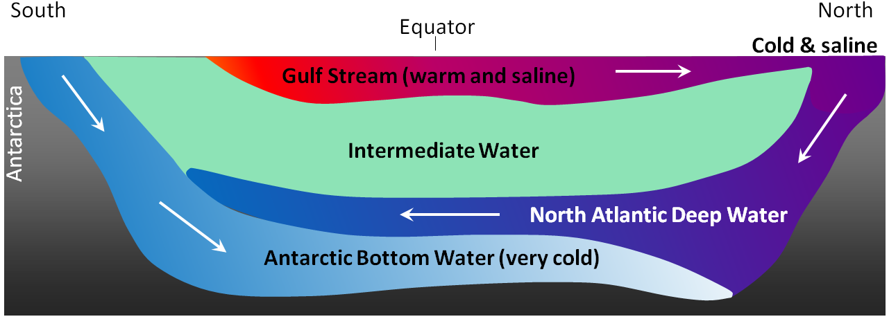
To see how this works, consider the warm and saline Gulf Stream current (Figure 16.10, top). It flows northward past Britain and Iceland into the Norwegian Sea, and cools as it moves north, becoming denser. Its high salinity contributes to its density, and it sinks, or downwells, deep beneath the surrounding water, forming the North Atlantic Deep Water (NADW) current that flows south. Meanwhile, at the southern extreme of the Atlantic, very cold water adjacent to Antarctica also sinks to the bottom to become the Antarctic Bottom Water (AABW) current. The AABW flows north, beneath the NADW.
_](figures/16-earth-system-change/figure-16-10.png)
Figure 16.10: A simplified north-south cross-section through the Atlantic Ocean basin showing the different current layers. Source: Steven Earle (2015) CC BY 4.0 view source
The water that sinks in the areas of deep water formation in the Norwegian Sea and adjacent to Antarctica moves very slowly at depth. It eventually resurfaces, or upwells, in the Indian Ocean between Africa and India, and in the Pacific Ocean, north of the equator (Figure 16.11).
_](figures/16-earth-system-change/figure-16-11.png)
Figure 16.11: Global thermohaline circulation patterns. Red lines are surface currents, and blue lines are deep currents. Source: NASA Earth Observatory (2008) Public Domain view source
Some ocean currents move warm water from the equator toward the poles. As in the example of the Drake Passage, the path of warm currents can have a significant impact on the climate of a region, and potentially of the planet as a whole. Processes that disrupt the density of seawater can slow or stop currents, preventing warm water from reaching higher latitudes. The recovery from the last ice age is characterized by sudden returns to glacial conditions over as little as 3 years. This is thought to be the result of enormous glacial lakes forming on continents as the glaciers melted, then being suddenly released into the ocean by a burst ice dam. The glacial water would be very cold, but it would also be fresh, making it less dense than the ocean water. The fresh glacial water would form a cap and slow the downwelling conveyor belt at high latitudes.
Scientists are trying to determine the current and past state of the Atlantic-basin system of circulation, called the Atlantic Meridional Overturning Circulation (AMOC), to tell whether it is changing in response to warming and adding fresh water from melting ice sheets. The AMOC varies considerably on decadal cycles because of cycles in the wind patterns in the Atlantic, so it is important to distinguish these cyclical changes from any longer-term underlying changes.
Because of these studies, we have an idea of what the physical properties of the Atlantic Ocean look like when circulation is stronger or weaker. When circulation slows, the density is lower in the downwelling regions (Figure 16.12, blue patch in the Labrador Sea). The density is higher south of this region, along the eastern coast of the United States and southern Canada (Figure 16.12, orange patch). Model simulations are used to confirm that the changes in density we observe are consistent with how we understand the circulation system to work.
Measurements of the actual flow rate at depth in the Atlantic Ocean (Figure 16.12, right, blue dots) confirm that density decreases in downwelling regions (black and red lines) when circulation slows. A more recent study (Caesar et al., 2018) has shown that observed and model temperatures follow the same pattern, with cooling where the blue patches are in Figure 16.12, and warming in the region of the orange patches. This is to be expected because the slowdown in circulation affects how heat is moved northward.
_](figures/16-earth-system-change/figure-16-12.png)
Figure 16.12: Using changing density to track circulation in the Atlantic Ocean. Left- Density calculated from measurements of temperature and salinity in a layer between 1,000 m and 2,500 m depth in the Labrador Sea (black box). Middle- Model results used to see what change in density can be expected. The model shows the same general relationship, with lower density in the Labrador Sea, and higher density to the south. Note that density units are in kg/m2 rather than kg/m3 because they are integrated over the layer. Right- Changing density in the Labrador Sea over time. Red and black lines show changes in density from two different data sets. In general, the peaks and troughs of these data sets match up. Blue dots are measurements of the rate of circulation from a project that began collecting data in 2004. See the References section for more information about the relevant studies. Source: Karla Panchuk (2018) CC BY-SA 4.0. Modified after Jon Robson (2013) CC BY-SA 4.0 view source
16.2.2.2 Is Atlantic Circulation Slowing Down More than Usual?
Changes in the Atlantic meridional overturning circulation (AMOC) happen from decade to decade. To know whether circulation is changing compared to what is normal, it is necessary to get information about what circulation looked like in the past. This is difficult to do, because measurements of circulation rates, temperature, and salinity don’t go back as far as we need them to.
In a new study, Thornalley et al. (2018) have used geochemical analyses of microfossils to build a longer-term record of temperatures, then used that record to look for the temperature “fingerprint” of slowing AMOC, an increasing difference in the temperatures of surface waters compared to deeper waters in the downwelling zone (Figure 16.13, top). They observe a longer-term cooling trend beginning at the close of the Little Ice Age, suggesting that less heat is being moved toward the downwelling zone (labelled A on the globe in Figure 16.13).
_](figures/16-earth-system-change/figure-16-13.png)
Figure 16.13: Long-term record of Atlantic Meridional Overturning Circulation (AMOC). Top- Temperature fingerprint of circulation determined using geochemical analyses of marine microfossil shells. Results show the difference between temperatures measured at depth at A on the globe, and temperatures measured near the surface at B. Cooling at A relative to B is indicative of weakening AMOC. Bottom- Changes in silt grain-size used to show changes in the velocity of currents at depth at C on the globe. A smaller average grain size means a slower current, and weaker AMOC. Source: Karla Panchuk (2018) CC BY 4.0. Modified after Thornalley et al. (2018). Locator globe modified after Reisio (n.d.) Public Domain view source
They also measured the size of silt grains on the sea floor, above which a southward-moving component of the AMOC system flows (location labelled C on the globe in Figure 16.13). Grain size is used as a substitute for a direct measure of ocean current velocity because the velocity determines what grain size can be carried. They identified a lower average grain size over the past ~150 years compared to the average grain size from earlier (Figure 16.13, bottom, dashed lines). The authors of the study note that the average grain size changes more during cold events in the Northern Hemisphere (the Dark Ages Cold Period and the Little Ice Age).
Thornalley et al (2018) conclude that the AMOC has been weaker on average during the past ~150 years than during the previous ~1,500 years. However, they cannot say for sure how much of that change is from melting that occurred at the close of the Little Ice Age, from melting triggered by warming since the Industrial Revolution, or some combination of the two. Direct measurements of density and current velocity tell us that as of 2017, the AMOC continues to weaken.
16.2.2.2.1 Plate Tectonics and Heat Transport
The opening of the Drake Passage is one example of how plate tectonic changes can affect ocean heat transport, and therefore climate. Plate tectonic changes that build or break up continents also play a role. When continents become large, ocean currents warm their margins, but the interiors can be much cooler. Anyone living on the Canadian prairies who has shivered through -40 °C temperatures in the winter, while watching news reports of rain in Vancouver will be familiar with this effect. When the supercontinent Gondwana was over the south pole approximately 300 million years ago (Figure 16.14), this triggered an ice age. The build-up of ice was hastened by the ice albedo feedback effect.
 Click the image for terms of use._](figures/16-earth-system-change/figure-16-14.jpg)
Figure 16.14: Glaciation on the supercontinent Gondwana. Paleogeographic reconstruction for 306 million years ago._ Source: C. R. Scotese, PALEOMAP Project (www.scotese.com) view source. Click the image for terms of use._
16.2.2.2.2 Short-Term Cycles in Heat Transport: El Niño Southern Oscillation
The El Niño Southern Oscillation (ENSO) operates on a much shorter timescale than climate forcings driven by plate tectonics or orbital cycles, alternating between El Niño and La Niña events on timescales of between two and seven years (Figure 16.15).
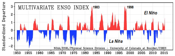. Modified after Klaus Wolter/ NOAA (n.d.) Public Domain [view source](https://www.esrl.noaa.gov/psd/enso/mei.ext/index.html)_](figures/16-earth-system-change/figure-16-15.png)
Figure 16.15: Variations in the ENSO index from 1950 to 2015. Source: Steven Earle (2015) CC BY 4.0 view source. Modified after Klaus Wolter/ NOAA (n.d.) Public Domain view source
Under normal conditions, strong winds blowing westward across the Pacific cause water to pile up in the western Pacific. This forces deeper colder water to the surface in the eastern Pacific (Figure 16.16, left). During La Niña events, further intensification of winds causes even more cold water to upwell. During an El Niño event, the winds weaken, allowing water to flow back to the east (Figure 16.16, right). The cold water settles deeper once again, meaning that warmer water is present along the eastern margin of the Pacific Ocean.
/ [El Niño](https://commons.wikimedia.org/wiki/File:ENSO_-_El_Ni%C3%B1o.svg)_](figures/16-earth-system-change/figure-16-16.png)
Figure 16.16: El Niño Southern Oscillation (ENSO) cycles are driven by changes in wind patterns that affect the distribution of warm and cold water in the Pacific Ocean. Source: Karla Panchuk (2018) CC BY 4.0. Modified after Fred the Oyster and NOAA/PMEL/TAO Project Office. View Normal Conditions/ El Niño
ENSO events affect weather on a global scale (Figures 16.17 and 16.18). In western Canada, El Niño years have warmer than average winters, whereas La Niña years have cooler than average winters.
_](figures/16-earth-system-change/figure-16-17.jpg)
Figure 16.17: El Niño climate impacts. Source: NOAA Climate.gov (n.d.) Public Domain view source
_](figures/16-earth-system-change/figure-16-18.jpg)
Figure 16.18: La Niña climate impacts. Source: NOAA Climate.gov (n.d.) Public Domain view source
16.2.3 Climate Forcing by Changes in the Atmosphere’s Energy Budget
Earth’s atmosphere regulates climate by controlling how much energy from Earth’s surface escapes to space, and how much of the sun’s energy reaches Earth’s surface.
16.2.3.1 Albedo
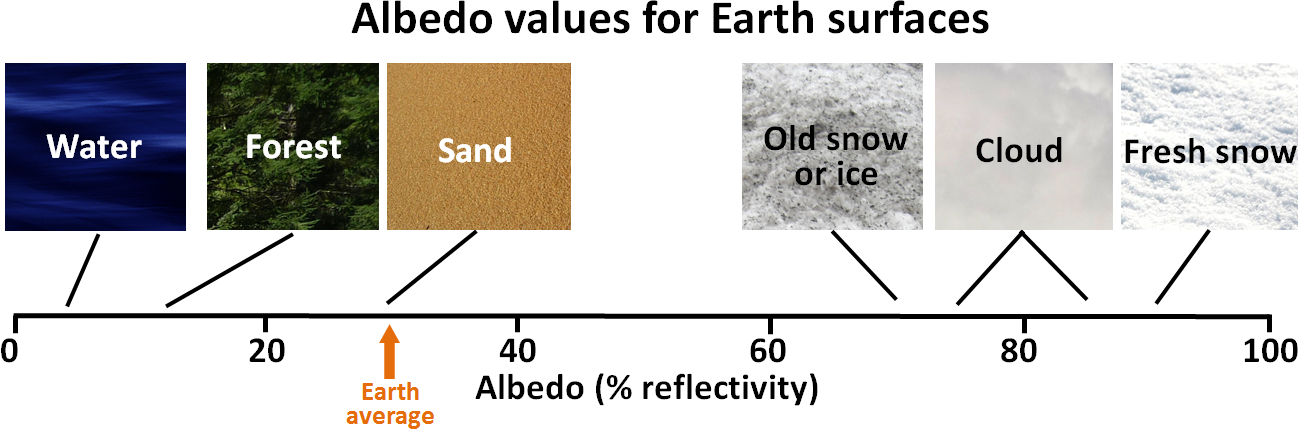
Albedo is a measure of the reflectivity of a surface. Earth’s various surfaces have widely differing albedos, expressed as the percentage of light that reflects off a given material. This is important because most solar energy that hits a very reflective surface is not absorbed and therefore does little to warm Earth. Water in the oceans or on a lake is one of the darkest surfaces, reflecting less than 10% of the incident light. Clouds and snow or ice are among the brightest surfaces, reflecting 70% to 90% of the incident light (Figure 16.19).
_](figures/16-earth-system-change/figure-16-19.png)
Figure 16.19: Typical albedo values for Earth surfaces. Surfaces with low values reflect less light than surfaces with high values. Source: Steven Earle (2015) CC BY 4.0 view source
Albedo, Feedbacks, and the Acceptance of Milanković Cycles as a Climate Forcing Mechanism
When Milanković published his hypothesis in 1924, it was widely ignored, partly because it was evident to climate scientists that the forcing produced by the orbital variations alone was not strong enough to drive the climate changes of the glacial cycles. Those scientists did not recognize the power of positive feedbacks. It wasn’t until 1973, 15 years after Milanković’s death, that sufficiently high-resolution data were available to show that the Pleistocene glaciations were indeed driven by the orbital cycles, and it became evident that the orbital cycles were just the first step, initiating a range of feedback mechanisms that made the climate change, many of which were related to albedo.
Consider the following:
- When large volumes of ice melt — such as the continental ice sheets of Antarctica and Greenland, as well as alpine glaciers— this decreases albedo. More solar energy is then absorbed by land, amplifying the increase in temperature.
- When sea ice melts and exposes water, the albedo of the exposed area decreases drastically, from approximately 80% to less than 10%. Far more solar energy can be absorbed by the water compared to the previous ice cover, amplifying the temperature increase.
- Sea level rises when ice and snow melt on land, and because seawater expands when heated. Higher sea level means a larger proportion of the planet is covered with water, which has a lower albedo than land. More heat is absorbed, amplifying the temperature increase. Since the last glaciation, a rise in sea level of approximately 125 m has flooded vast areas of land.
Exercise: Albedo Impacts of Vegetation Changes
Changes in climate can cause forests to be replaced by grasslands, which have higher albedo than dark forest cover. If deserts expand, vegetated areas can be replaced by higher-albedo sand. Many human activities affect albedo, including adding urban surfaces to an environment, and planting crops. Figure 16.20 shows a forest that has been clear-cut. If a clear-cut has an albedo similar to that of sand, how would clear cutting change the albedo of the area?
_](figures/16-earth-system-change/figure-16-20.jpg)
Figure 16.20: A clear-cut near Eugene, Oregon. Source: Calibas (2011) CC BY-SA 3.0 view source
Note that trees cool their environment through transpiration, when they release water vapour from their leaves. Changes in local temperatures when trees are clear-cut also include the effects of reduced evaporative cooling. Changes in vegetative cover also affect the rates of CO2 uptake by plants.
16.2.3.2 Greenhouse Gases (GHGs)
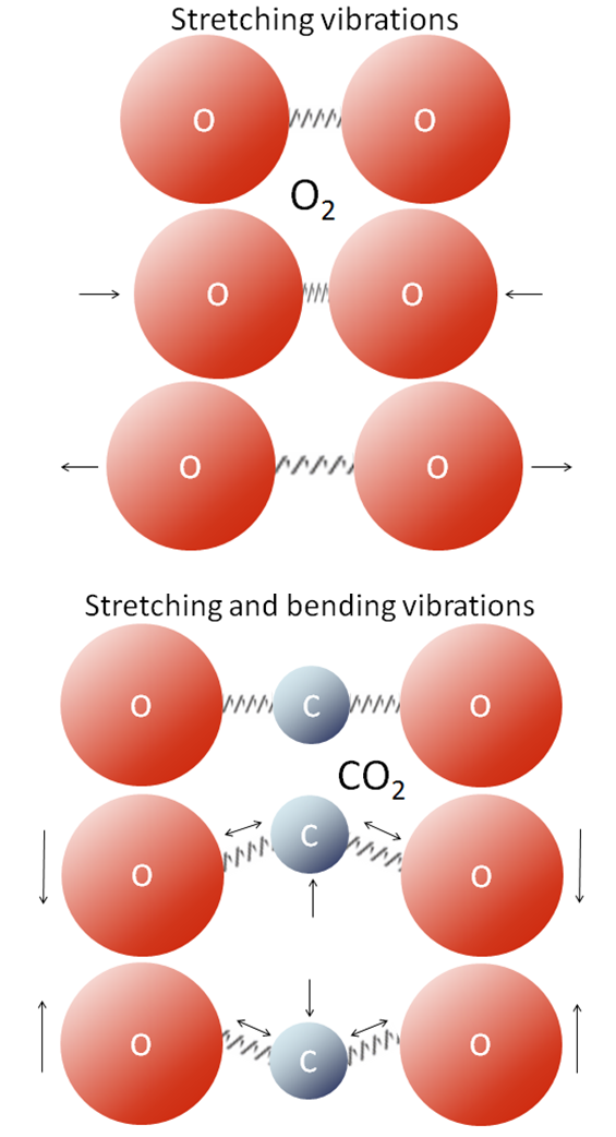
All molecules vibrate at various frequencies and in various ways, and some of those vibrations take place at frequencies within the range of the infrared radiation that is emitted by Earth’s surface. Gases with two atoms, such as O2, can only vibrate by stretching (back and forth; Figure 16.21 top), and those vibrations are much faster than that of IR radiation. Gases with three or more atoms (such as CO2) can vibrate in other ways, such as by bending (Figure 16.21 bottom). Those vibrations are slower and allow the molecules to absorb and release infrared radiation.
_](figures/16-earth-system-change/figure-16-21.png)
Figure 16.21: Molecules with two atoms (top) vibrate differently from molecules with more than two (bottom), and this determines whether a gas will be a greenhouse gas or not. Source: Steven Earle (2016) CC BY 4.0 view source
When infrared radiation interacts with CO2 or with one of the other GHGs, the molecular vibrations are enhanced because there is a match between the wavelength of the light and the vibrational frequency of the molecule. This makes the molecule vibrate more vigorously, heating the surrounding air in the process. These molecules also emit infrared radiation in all directions, some of which reaches Earth’s surface. Heating due to the vibrations of greenhouse gas molecules is called the greenhouse effect. Water molecules (H2O), and methane molecules (CH4) also interact with infrared radiation when they vibrate, so they are greenhouse gases as well.
Ice core records show that over the last 800,000 years, rapid cycles into and out of glacial temperatures are associated with similarly-timed cycles in atmospheric CO2 levels (Figure 16.21).
. The dashed line shows a recent measurement of atmospheric CO~2~ levels from the Mauna Loa Observatory. [Click to view the latest measurements](https://scripps.ucsd.edu/programs/keelingcurve/). Bottom: Temperature record derived from oxygen isotope measurements of water in ice cores. [Data from Jouzel et al (2008).](https://www.ncdc.noaa.gov/paleo-search/study/6080) Upper dashed line- global surface temperature for 2016 from NASA's Goddard Institute for Space Studies Reference line. [Click to view the most recent anomaly](https://climate.nasa.gov/vital-signs/global-temperature/). Lower dashed line: average temperature for the past 1000 years. _Source: Karla Panchuk (2018) CC BY 4.0, modified after National Research Council (2010) [view source](https://nas-sites.org/americasclimatechoices/more-resources-on-climate-change/climate-change-lines-of-evidence-booklet/evidence-impacts-and-choices-figure-gallery/#jp-carousel-736). Click the image for terms of use._](figures/16-earth-system-change/figure-16-22.png)
Figure 16.22: Variations in atmospheric CO2 levels and temperature over the last 800,000 years. Top- CO2 concentration from ice core data in Lüthi et al (2008). The dashed line shows a recent measurement of atmospheric CO2 levels from the Mauna Loa Observatory. Click to view the latest measurements. Bottom: Temperature record derived from oxygen isotope measurements of water in ice cores. Data from Jouzel et al (2008). Upper dashed line- global surface temperature for 2016 from NASA’s Goddard Institute for Space Studies Reference line. Click to view the most recent anomaly. Lower dashed line: average temperature for the past 1000 years. Source: Karla Panchuk (2018) CC BY 4.0, modified after National Research Council (2010) view source. Click the image for terms of use.
16.2.3.2 Earth-System Response Time
You might have noticed that for most of the 800,000-year record in Figure 16.22, there is a fairly consistent relationship between scale of change in atmospheric CO2 levels and the resulting change in temperature. You might also have noticed that compared to most of the record, the rise in temperature since 1950 is unexpectedly small, given the increase in atmospheric CO2 levels since that time. The reason for the relatively small temperature increase in response to the recent CO2 increase is in large part because the recent rise in CO2 is happening far more rapidly than other parts of the Earth system can respond. The ocean in particular is slowing down the response.
The ocean takes up heat from the atmosphere, and thus helps to determine surface temperatures. A relatively cool ocean can take up more heat from the atmosphere, reducing warming. The fastest way for the ocean as a whole to take up heat is through the “stirring” that happens with ocean circulation, but circulation happens on thousand-year timescales. The slow rate of circulation means that centuries from now, there will still be cool water rising up from the deep ocean that has yet to be exposed to the warmer surface conditions. At other times in the 800,000-year record, changes in CO2 levels happened on timescales much closer to those at which the ocean takes up heat.
16.2.3.3 Atmospheric Effects of Volcanic Eruptions
Volcanic eruptions don’t just involve lava flows and exploding rock fragments. Eruptions also release particles and gases into the atmosphere. Important volcanic gases include water vapour, CO2, and sulphur dioxide (SO2). Volcanic CO2 emissions can contribute to climate warming if a greater-than-average level of volcanism is sustained over a long time. At the end of the Permian Period, the massive Siberian Traps were produced by eruptions lasting at least a million years. Large quantities of CO2 were released, warming the climate and triggering a cascade of Earth-system responses. The end of the Permian Period at 252 Ma is marked by the greatest mass extinction in Earth history.
Over the shorter term, however, volcanic eruptions can have the opposite effect, cooling the climate. SO2 reacts with water in the atmosphere to make droplets of sulphuric acid. The sulphuric acid droplets scatter sunlight, reducing how much of the sun’s energy can reach Earth’s surface. They also affect cloud formation. The volcanic cooling effect is relatively short-lived, because the particles settle out of the atmosphere within a few years.
Exercise: Climate Change at the end of the Cretaceous Period
The large extraterrestrial impact at the end of the Cretaceous Period 66 Ma ago is thought to have produced a massive amount of dust, which may have remained in the atmosphere for several years. It may also have produced a great deal of CO2. What do you think would have been the short-term and longer-term climate-forcing implications of these two factors?
16.3 Methods for Studying Past Climate
Whereas weather refers to day-to-day variations in temperature, precipitation, winds, and so on, climate refers to long-term trends in weather patterns (over decades or more). The term __paleoclimate __refers to Earth’s climate in the past. The information we have about Earth’s past climates can be classified as direct data or proxy data. Direct data are information derived from first-hand observations of climate. Direct data can be instrumental data, derived from tools designed to quantify observations, or from qualitative descriptions.
__Proxy data __are information derived from natural materials with characteristics that are affected by climate in a systematic way. This could also be said of some instrumental data: an alcohol thermometer uses the fact that the volume of alcohol changes in a consistent way in response to temperature. Proxy data rely on relationships that are also as systematic and consistent, but there are important differences:
- Instruments are designed so that the response of the instrument reflects only one characteristic of the environment (e.g., an alcohol thermometer is sealed so that only temperature affects the level of alcohol, not air pressure or evaporation), but proxy data may need to be carefully analyzed to account for other processes.
- Data from instruments are lost if observations are not made and recorded. A thermometer is constantly changing in response to temperature, and will not stay in a particular state once conditions change. Proxy records capture information about the environment in a way that can persist over the long term, for as long as the materials last in usable form. Some proxy records preserve information from billions of years ago.
- Instruments transform characteristics of the environment into information that we can access immediately (e.g., you can read a temperature directly from a thermometer), but materials from which we derive proxy data require processing, often with specialized laboratory equipment, to get data we can use.
- Instruments measure only what we design them to measure, and measure only as well as we design them to do so. Because proxy data come from materials that persist through time, it is possible to improve the techniques used to analyze materials, and redo earlier measurements. Discovering new proxies is an ongoing area of research, and regularly reveals ways to determine characteristics of past states of the Earth system that we didn’t think were knowable.
- Instrumental records and other direct observations can be well constrained in time. In other words, we often know the exact dates the observations were made. Proxy data may come from materials that are difficult to pin down to an exact date, and additional information may be required to determine when the records were formed. Sometimes proxy data can only be extracted as an average over a number of years. The relevant question becomes whether the resolution of the record (how detailed it is) is high enough for the time frame of interest. For example, an annual average would be no use at all to understand monthly climate variations, but would provide exceptionally high resolution for geological processes operating over tens of thousands of years.
16.3.1 Types of Direct Data
Instrumental records of climate are those derived from tools such as thermometers, rain gauges, or satellite measurements of the extent of ice sheets. Instrumental records are a recent development, as the history of the Earth system goes. The oldest known temperature measurements cover the period from 1654 to 1670, and were made by monks and Jesuit priests who operated stations within a meteorological network supported by the Medici family of Florence.
Non-instrumental historical records of climate also exist, and cover periods of human history prior to the development of the climate-measuring tools we have now. With detective work, these can be used to paint a detailed picture of past climates. Non-instrumental historical records include written records about how long ice and snow were present in a particular year, when harvests occurred, when floods happened, and shipping records that report the extent of sea ice. Paintings of alpine glaciers give information about how far the ice extended, and this can be used to reconstruct temperatures.
16.3.1 The Challenges of Getting Climate Information from Historical Records
In their paper Historical Climate Records in China and Reconstruction of Past Climates, Jiacheng Zhang and Thomas Crowley used official Chinese records extending as far back as 1000 CE to get a detailed picture of climate. This involved transforming descriptions of weather events into a systematic scale. One challenge is defining the scale, but another is deciding what individual accounts actually mean. The authors point out that records of rain or drought can reflect the perceptions and generalizations of the people who wrote about the weather, rather than what actually happened. Consider the following description of rainfall in 1644 from Diary of Qi Zongmin:
“in Wyzhong there is no rain for six months from May”
Does this mean there was no rain at all prior to May, or just very little? Was it actually six months since there had been rain, or is that an approximation? How do we reliably translate different systems of time measurement into durations and dates, like “six months” or “May?” How can we tell for sure where a location is if place names or political boundaries change?
As the authors caution, “a great deal of cross-checking [is required] in order to arrive at a useful descriptive account of climate anomalies.”
16.3.2 Sources of Proxy Data
16.3.2.1 Tree Rings
The study of tree growth rings for the purpose of understanding past states of the Earth system is called dendroclimatology. Temperatures and a history of drought or wet periods can be reconstructed from the widths of tree rings. Because tree rings form annually, these records can also be well constrained in time. The widths of tree rings reflect how fast the tree grows in a given season. There are factors other than temperature and moisture that affect growth rate, so a sampling strategy must be carefully designed to ensure confidence in climate reconstructions.
16.3.2.2 Stable Isotopes
Atoms have a nucleus made of protons and neutrons. The number of protons in the nucleus determines what element the atom is, and will always be the same for a given element. In contrast, the number of neutrons can vary for an element. Versions an element having different numbers of neutrons are the isotopes of that element.
Sometimes an atom has a number of neutrons that makes it unstable. Those atoms eventually break apart, releasing energy, and are called radioactive isotopes. The decay rate of radioactive isotopes is known, making it possible to use them to find the ages of natural materials. For example, carbon-14 dating makes use of the radioactive isotope of carbon, 14C, which has eight neutrons instead of the usual number, six (the 14 refers to 6 protons + 8 neutrons).
For investigating Earth’s past climate, stable isotopes, which do not decay, are used instead. Stable isotopes of the same element are measured in natural materials, and their ratios compared. Both isotopes are involved in the same chemical reactions and physical processes, but the slight difference in mass caused by one or two extra neutrons means that those processes are more likely to take up the lighter isotope than the heavier one. Some processes do this in such a particular way that evidence of their occurrence is left behind as a distinctive fingerprint in the stable isotope composition of materials formed in their environment.
The pair of isotopes used to reconstruct past temperatures are the oxygen isotopes 16O and 18O. The ratio of 18O to 16O in water is reflected in the calcium carbonate of shells that form in the water. The shells may remain in the geologic record long after the water is gone, making it possible to know the oxygen isotope compositions, and thus temperatures, of water bodies that existed in the distant past.
16.3.2.3 Ice Cores
The ice in polar glaciers and mountain glaciers preserves a detailed snapshot of Earth’s atmosphere and climate. A sample of Earth’s atmosphere, including gases and particles, is captured and held within the ice, and buried beneath subsequent ice layers. The annual layers in the ice can be used to determine a timescale for the data. The gases in air bubbles trapped within ice (Figure 16.23) are analyzed to determine the chemical composition of the atmosphere at the time the gasses were trapped.
_](figures/16-earth-system-change/figure-16-23.jpeg)
Figure 16.23: A researcher holds a fragment of ice from Antarctica. The dots in the fragment are air bubbles containing samples of Earth’s past atmosphere._ Source: Atmospheric Research, CSIRO (2000) CC BY 3.0 view source_
Ice cores (Figure 16.24) are cylinders of ice retrieved using a specialized drill bit. The cores are carefully packaged and stored in specially designed facilities (Figure 16.25) until they are analyzed.
_](figures/16-earth-system-change/figure-16-24.jpg)
Figure 16.24: A scientist weighs and measures a cylinder of core from the West Antarctic Ice Sheet before she packages it for transport. Source: NASA/Lora Koenig (2010) CC BY 2.0 view source
 in Lakewood, Colorado. Ice cores are housed in tubes 1 m long. The main storage facility is kept at -36 ºC. Fortunately, scientists can examine the cores under much warmer conditions in a nearby room maintained at -24 ºC. _Source: U. S. Geological Survey/ Eric Cravens (n.d.) Public Domain [view source](https://commons.wikimedia.org/wiki/File:NICL_Freezer.jpg)_](figures/16-earth-system-change/figure-16-25.jpg)
Figure 16.25: National Science Foundation Ice Core Facility in Lakewood, Colorado. Ice cores are housed in tubes 1 m long. The main storage facility is kept at -36 ºC. Fortunately, scientists can examine the cores under much warmer conditions in a nearby room maintained at -24 ºC. Source: U. S. Geological Survey/ Eric Cravens (n.d.) Public Domain view source
16.3.2.4 Rock and Fossil Distributions
Earth can be divided into six main climate zones (Figure 16.26). The zones run roughly along lines of latitude, so that the climate zone changes as you move north or south of the equator. When the climate warms, the zones shift away from the equator; an area now in the boreal climate zone might have been in the warm temperate climate zone when Earth’s climate was warmer. When the climate cools, the zones shift toward the equator.
_](figures/16-earth-system-change/figure-16-26.png)
Figure 16.26: Six climate zones of the Köppen-Geiger classification. Source: Karla Panchuk (2018) CC BY-SA 4.0. Modified after LordToran (2007) CC BY-SA 3.0 view source
Some rock types are characteristic of particular climate zones. For example, coal deposits are characteristic of a subtropical climate. Limestone with coral reef fossils is characteristic of a tropical climate. If a rock type is found outside of its climate zone, that might indicate a change in climate. Coal can be found near Estevan, Saskatchewan, now in the warm temperate climate zone. This suggests that at one time, a warmer climate resulted in a northward shift of the subtropical climate zone. Some of the oil in western Canada is present in pore spaces within ancient coral reefs. The warm temperate climate zone cannot have been at its present location when those reefs formed.
Fossils can be used similarly. If an organism lives in a habitat with a particular climate, then evidence that the organism has migrated away from the equator could indicate warming. Migration toward the equator could indicate cooling.
The study of pollen and plant spores, called palynology, is very helpful for determining the distribution of plants when evidence of larger plant parts (e.g., fossil leaves and bark) is absent. Pollen and spores are very tough, and will survive in the environment when other plant materials do not. A detailed record of pollen and spores, and hence of the climate zones in a particular location, can be derived from lake sediments. Lakes in climates with strong seasonality (a distinct difference in temperature as seasons progress) can accumulate distinct annual sediment layers, called varves (Figure 16.27). Each year is represented by a light layer and a dark layer. The light layers consist of sand and silt from spring runoff. The darker layers include organic matter accumulated during the year.
. Click the image for terms of use._](figures/16-earth-system-change/figure-16-27.png)
Figure 16.27: Varves in a core from Canoe Brook, Drummerston, Vermont. Each pair of light and dark layers represents one year. The top of the core is to the right. Source: Karla Panchuk (2017) CC BY-NC-SA 4.0 (labels added). Modified after Jack Ridge/ North American Glacial Varve Project (2008) view source. Click the image for terms of use.
Varves can be counted to determine the age of the sediment, and the pollen and spores within the sediment can be extracted to see what types of vegetation were present at different times.
16.4 Computer Models of the Earth System
Earth-system interactions are so complex that it is next to impossible to follow all of the connections and implications without help. So, scientists use Earth-system computer models to assist. Earth-system models incorporate knowledge of the many components of the Earth system in a way that makes it possible to test how important any one change is.
Earth-system models vary in how many aspects of the Earth system they include, and how detailed their representations of those aspects are. Models are designed to answer particular kinds of questions so their performance can be optimized; a study that is concerned only with large-scale global changes might not require a model with a highly detailed representation of Earth’s coastlines. It takes more time to run a complicated model, so this saves on computing resources.
When computer models are discussed, we acknowledge that there is a difference between measurements of the real world, and the output from the model. Modelers are careful to refer to measurements of the real word as data, and output from the model as results. This also helps to avoid confusion when comparing models to real-world measurements to gauge how realistic the model output is.
16.4.1 What Are Computer Models, Exactly?
Computer models describe natural phenomena using mathematical equations. On the most basic level, computer models take some quantity—whether heat, water, or the concentration of a pollutant—and calculate how it moves through a system. Sometimes they look only at how that quantity changes through time. A computer model of the water volume in a bathtub could be limited to looking at how rapidly water flows in through the tap, and how rapidly it flows out through the drain. But sometimes models look at how a quantity changes in space as well as through time.
A study of wind-driven currents in a lake must include information about the shape and depth of the lake to capture how friction at the lake bottom and along the sides affects water flow (Figure 16.28). Data about the lake shape and depth (Figure 16.28, top) is translated to a model grid (Figure 16.28, bottom). Calculations are done to see how wind and friction control how water moves into and out of each cell in the grid.
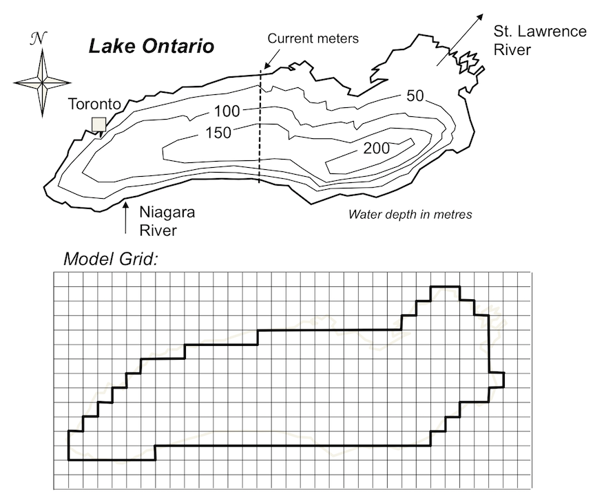
Figure 16.28: Set-up for a model of wind-driven current flow in Lake Ontario. Top: Map of Lake Ontario showing water depth and the location of current meters. Bottom: Grid used to translate water depth information for model calculations. Source: Karla Panchuk (2002) CC BY 4.0. Based on the exercise described in Chapter 10 of Slingerland & Kump (2011).
The model produces information about wave height (Figure 16.29, left) and shows the direction and speed of water flow across the lake using arrows of different sizes (Figure 16.29, right). If scientists are interested in how a pollutant would move around the lake, they can include the location where the pollutant is added, and how rapidly it is added, and track how it moves.
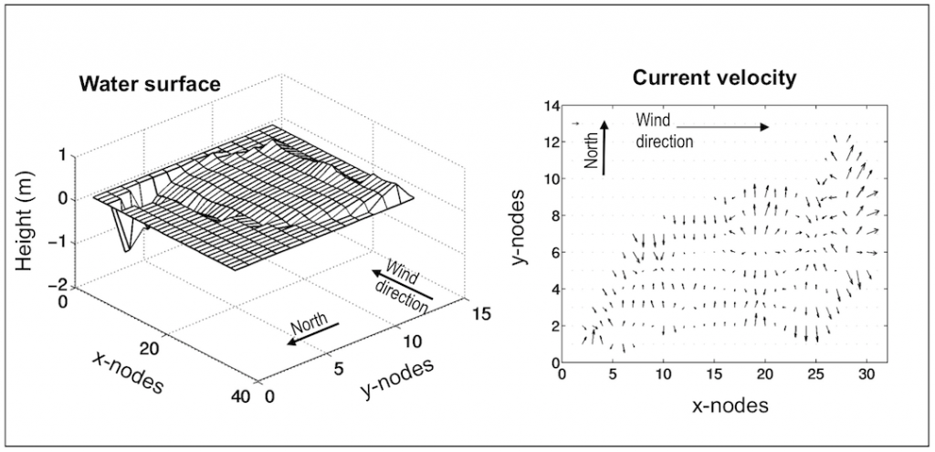
Figure 16.29: Height of the water surface (left) and current velocity (right) from a model of wind-driven flow in Lake Ontario. The length of current arrows shows the speed of the current, and the arrow points in the direction of flow. Source: Karla Panchuk (2002) CC BY 4.0. Based on the exercise described in Chapter 10 of Slingerland & Kump (2011).
If the model is to be used to track the movement of a pollutant through the lake, it is important to know that it has done a good job of calculating the current velocity. In this case, data from current meters in the lake can be compared to the current velocities that the model calculates (Figure 16.30). The model captures the fact that flow is northward near the margins of the lake, and southward in the middle, but the model current velocities are not exactly the same. This means that the model would do a good job of predicting where the pollution went, but not as good a job at predicting how fast it got there.
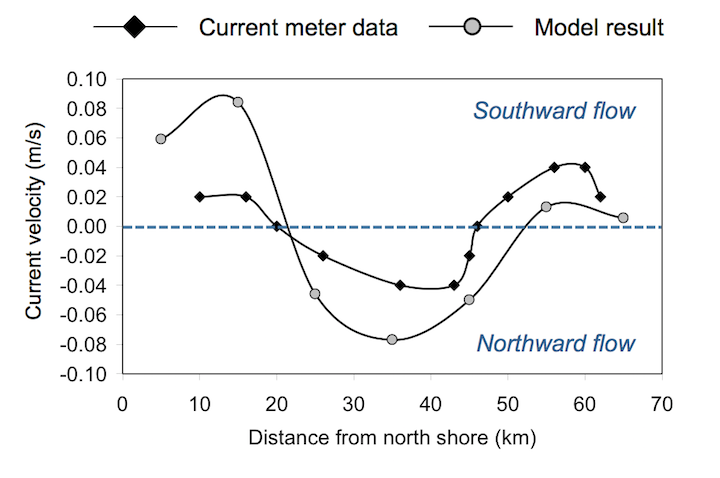
Figure 16.30: Comparison of model results with current meter data. Points plotted beneath the blue dashed line indicate northward flow. Points above indicate southward flow. Source: Karla Panchuk (2002) CC BY 4.0. Data from Simons and Schertzer (1989).
The model in this case had a relatively course representation of the lake geography, so a first step would be to make the grid cells smaller to do a better job of simulating the shape of the lake, then look at the flow in finer detail. Another step would be to represent the lake water using a vertical stack of several grid cells to better capture the extent to which bottom friction and wind force affect the lake water at different depths, and to do a better job of representing the water depth.
16.4.2 An Example of Using a Computer Model to Study Past Earth-System Change
The Paleocene-Eocene Thermal Maximum (PETM) was a sudden global warming event that happened approximately 56 million years ago. There was interest in studying this event because its suddenness was thought to be a good analogy for the rapid changes happening in the Earth system today. Cores from ocean-floor rocks show that the oceans became so acidified during the PETM that calcium carbonate sediments dissolved over vast areas of the ocean floor, vanishing entirely from some regions. The same cores also showed a shift in the carbon-isotope composition of calcium carbonate sediments.
Both the acidification and the carbon-isotope shift indicated that a large amount of carbon was added to the Earth system to trigger the PETM. The problem was that there were a number of possible sources for the carbon, and thus a number of possible triggers for the event. Although scientists provided reasoned arguments for their favourite hypotheses, there was no way to know for sure which was the best answer.
To solve this problem, an Earth-system model was used that could test which scenario could best account for the pattern of dissolving calcium carbonate. It took into account the shape of ocean basins, ocean current circulation, and carbonate system chemistry in ocean water and in sediments. It also took into account changes in sediments once they were deposited.
The steps to using this model were the following:
- A search was done to locate as many studies of ocean floor sampling sites as possible that had information about changes in the amount of calcium carbonate during the PETM.
- The model was set up so that it did a good job of reproducing the distribution of calcium carbonate before the PETM happened. This was important to ensure that model scenarios began with a realistic set of conditions.
- Each of the possible scenarios involved carbon coming from different sources in the Earth system, meaning that each scenario could be represented in the model by adding to the atmosphere different amounts of carbon with different carbon isotope compositions. The more carbon a scenario required, the more the calcium carbonate sediments would have dissolved in real life.
- The model was run for each different amount of carbon. For each scenario, the pattern of calcium carbonate sediments that the model gave was compared to the actual distribution of calcium carbonate sediments known from the data collected in Step 1. In the end, the model showed that some of the scenarios did not even come close to matching the observations, either dissolving way too much calcium carbonate, or far too little. The model showed that two scenarios did come close to reproducing the pattern of calcium carbonate, and that one did a better job of matching the observations than the other. When it came time to write a report about the experiments, the scientists learned that newly published measurements from another study supported the scenario that the model suggested was best. It would have been acceptable to write a paper describing the model results, and which scenario worked best. However, also being able to comment about new supporting data meant there was a better chance of convincing other scientists that the model results were meaningful.
16.4.3 Predicting the Future of the Earth System with Models
Using models to investigate the Earth system requires careful consideration of how to build the model and run experiments. But it also requires skillful use of real-life measurements to set up the model, and to interpret and evaluate its results. The PETM model study was an example of how a model can be used to test hypotheses about past behaviour of the Earth system. There were data from before, during, and after the event to help set up the model and gauge its effectiveness.
Using Earth-system models to predict the future is a different kind of modeling challenge, because we don’t already know what the right answer is. The situation being modeled hasn’t happened yet. Scientists who try to predict the future of the Earth system have to do things a bit differently in order to have some confidence in the reliability of their model outcomes:
- They must come up with reasonable forcing scenarios for the model. A model used to predict the future of Earth’s climate will need input about what atmospheric greenhouse gas levels will be. That will depend on what actions humans take. Scientists deal with this unknown variable by testing multiple scenarios for greenhouse gas levels, such as what would happen if fossils fuels continue to be used as they have been, or alternatively, what would happen if we completely stopped using fossil fuels tomorrow. The scenarios they choose span a range of possibilities, including extreme cases, to make sure they understand what the possible range of outcomes could be.
- Scientists use some of the data they have to set the model up so that it is a realistic representation of the Earth system at a particular time in history. They then test the model to see if it can reproduce a different set of data later in history. This is a way to see if the model can get the right answer for a time when we know the right answer. Finally, after determining that the model gives reasonable results for times when we know the right answer, it is run for future scenarios.
- To be confident about predictions of future Earth-system change, scientists may collaborate to run their scenarios on many different Earth-system models designed by many different research groups at many different institutions. These models are set up with slightly different mathematical representations of processes, or different levels of detail in geographic representations. The scientists who built the various models might disagree on what numbers to assign some of the variables, or even which parts of the Earth system are necessary to include. If all the models produce similar results for a particular scenario in spite of representing a wide range of ideas about how such models should work, scientists can be more confident in those results.
- Scientists report uncertainty with their model results. It is a common misconception that uncertainty means the same thing as in everyday language—that we just don’t know something, or can’t say for sure. But for models, uncertainty is a number that indicates the likelihood that a model result is within a certain range of values. It is determined using methods that are themselves the product of careful research. A meaningful discussion of uncertainty will concern a specific model or set of models, a specific variable, and include a specific range of values. It will also include information about how large the uncertainty is compared to the changes they are investigating. If these details are missing from the conversation, it’s a clue that “uncertainty” is being used in a common-language way rather than the way that modellers use it. Note that reporting uncertainty is not exclusive to models predicting the future, but it is particularly important for those models because of the great scrutiny Earth-system models receive when they are used to investigate future climate change.
16.5 Humans in the Earth System
16.5.1 The Start of Human Influence on the Earth System
Anthropogenic change in the Earth system is change caused by humans. Many discussions of anthropogenic climate-change place the start of human impacts on the Earth system at the beginning of the industrial era, in the mid 18th century. The industrial era was when humans began to use fossil fuels—at the time, mostly coal—on a much larger scale than before to do things like run manufacturing machinery and trains.
Some climate scientists place the first anthropogenic impacts much earlier, however. Some suggest that anthropogenic climate change began around 8,000 BCE when humans cleared land for agriculture in Europe and the Middle East. Clearing forests for crops is a type of climate forcing because the CO2 storage capacity of the crops is generally lower than that of the trees they replace. Some climate scientists also point to the creation of wetlands to grow rice in Asia around 5,000 BCE. Creating wetlands is a type of climate forcing because the anaerobic bacterial decay of organic matter within wetlands produces CH4.
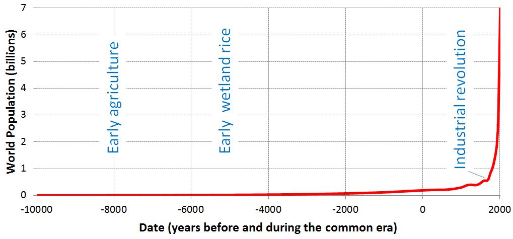
Whether anthropogenic climate change began with the Agricultural Revolution or the Industrial Revolution may be a matter for debate for some, but it is clear that Earth-system change accelerated once the Industrial Revolution began. Part of this is due to the fact that agricultural activities had to be scaled up to feed an ever-growing population. When humans first started growing crops, the world population was approximately 5 million (Figure 16.31), fewer people than live in Toronto today. The world population rose to approximately 18 million when wetland rice cultivation began (fewer people than live within the city limits of Beijing today), to over 800 million at the start of the Industrial Revolution. The world population was estimated at 7,600 million in 2018.
. Data from Roser and Ortiz-Ospina (2018) [view source](https://ourworldindata.org/world-population-growth)/ [view data file](https://ourworldindata.org/wp-content/uploads/2013/05/WorldPopulationAnnual12000years_interpolated_HYDEandUNto2015.csv)_](figures/16-earth-system-change/figure-16-31.png)
Figure 16.31: World population growth over the past 12,000 years. Source: Steven Earle (2015) CC BY 4.0, view source. Data from Roser and Ortiz-Ospina (2018) view source/ view data file
The other reason humans accelerated Earth-system change after the start of the industrial era is that human activities required a source of energy, and fossil fuels such as coal and oil were that source. Fossil fuels are those derived largely from plant material that grew, died, and was partially preserved at various times throughout Earth history. The plants removed CO2 from the atmosphere when they were alive, and stored it in organic compounds in their tissues. The materials accumulated over hundreds of millions of years in settings like swampy forests, shallow seas, and deltas. When fossil fuels are burned, the stored carbon is released back into the atmosphere as CO2.
16.5.2 The Carbon-Isotope Fingerprints of Fossil Fuel
Carbon isotopes provide insights into the extent to which fossil fuels have impacted the Earth system, because fossil fuels have a unique carbon-isotope fingerprint that is detectable in the atmosphere and in geological materials.
16.5.2.0.1 Stable Carbon Isotopes (12-Carbon and 13-Carbon)
When plants transform CO2 into tissues, the process imparts a unique carbon-isotope signature to the resulting organic matter. Plants preferentially take in CO2 with the isotope 12C over CO2 with isotope 13C. They do so in a consistent way, giving plant tissues a distinctive ratio of 13C to 12C. Fossil fuels are derived from plant materials, and they preserve this isotopic ratio.
The ratio of 13C to 12C is commonly expressed relative to a standard to give numbers that are easy to work with and compare. The notation δ13C refers to the ratio of 13C to 12C in a sample compared to the ratio in a standard, and is expressed in parts per thousand (or per mil, ‰). The standard has a δ13C of 0‰. Carbon in plant tissues has a δ13C of -25‰ to -30‰, meaning it has a 13C to 12C ratio that is 25 to 30 parts per thousand lower than the standard. Burning fossil fuel releases CO2 with that ratio into the atmosphere.
For most of the past 1000 years, the atmosphere has had a δ13C of approximately -6.5‰. The carbon-isotope composition of organic matter is much lower than that of the atmosphere, so the mixing in of carbon from fossil fuels causes the over-all carbon-isotope composition of the atmosphere to decrease. An analogy for mixing low δ13C CO2 into the atmosphere is rapidly adding cold water to a hot bathtub. The faster the cold water is added, the faster the bathwater will cool. The colder the water being added, the faster the bathwater will cool. In this analogy, the atmosphere is the bathtub, and fossil fuels are the water being added. The low δ13C value of fossil fuels (-25‰ to -30‰) is like very cold water being added.
As we would expect, the carbon isotope composition of the atmosphere takes a sudden downward turn at the same time that humans undertake the Industrial Revolution, and begin burning large quantities of fossil fuels, adding CO2 to the atmosphere at an accelerating rate (Figure 16.32).
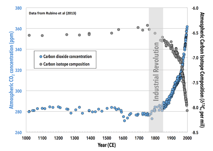
Figure 16.32: A 1000-year record of atmospheric CO2 levels (blue circles) and carbon isotope composition (grey circles) measured in Antarctic ice cores. The Industrial Revolution (grey shading), marking the start of the industrial era and the large-scale use of fossil fuels by humans, coincides with a sudden rise in CO2 levels, and a fall in the carbon-isotope composition of atmospheric CO2. Source: Karla Panchuk (2018) CC BY 4.0. Data from Rubino et al (2013).
Scientists who study past climates on Earth are familiar with carbon-isotope records like this one, because such records are used to reconstruct major changes in the Earth system through their impact on the carbon cycle. In carbon-isotope records from the distant past, a shift of more than 1.5‰ would be enough to catch the attention of a researcher and make them wonder what could have happened.
What is unusual about the 1.5‰ drop today in comparison to those observed in the geological record is how rapidly it is happening. It is more common to see such changes happen over millions of years, not hundreds of years. The rate at which atmospheric CO2 δ13C is dropping is approximately 10 times faster than the carbon-isotope shift at the PETM, which is the fastest event ever documented in the rock record.
Carbon dioxide in the atmosphere mixes into the oceans, where organisms take up carbonate ions to make calcium carbonate shells. The 1.5‰ drop has been imprinted in the calcium carbonate of marine organisms like sponges (Böhm et al, 2002), and will remain in the rock record globally, as evidence of human activity. Because of this, and because of many other such markers that are being left in the rock record by human activities (the presence of plastic, for example), some have suggested that it is time to define a new division of geological time, the Anthropocene Epoch. The start of the Anthropocene Epoch would mark the point at which human activities became evident in the geological record.
16.5.2.0.2 Radioactive Carbon (14-Carbon)
Carbon-14 dating relies on the fact that 14C decays to 14N at a known rate. By knowing the rate, and how much 14C and 14N are present, we can work out how long the decay has been happening. Knowledge of the decay rate of 14C also makes it useful to track fossil fuel additions to the atmosphere.
The rate of decay of a radioactive isotope is expressed as a half-life, which in this case is the amount of time it would take half of the 14C atoms in a sample to decay to 14N. The half-life of 14C is 5,730 years. After 10 half-lives, or 57,300 years, there isn’t enough 14C left to do an age measurement. Fossil fuels are millions to hundreds of millions of years old, long enough for there to be none of the 14C originally contained by the plant material.
There is a notation system for 14C similar to the δ13C notation system for the ratio of 13C to 12C, in which the amount of 14C is compared to a standard. Carbon-14 amounts are reported as Δ14C values in units of ‰. In that system, the atmosphere as a whole had a Δ14C of 45‰ in 2010, and fossil fuels have a Δ14C of -1000‰. Effectively, the atmosphere appears to be aging rapidly. In the bathtub analogy for carbon isotopes, adding CO2 from fossil fuels is like dumping ice into the tub.
The effects of fossil fuel CO2 on atmospheric Δ14C levels must account for 14C being made through natural processes in the atmosphere, and decaying away; for the decay of a large pulse of 14C created by nuclear bomb tests; and for other sources of carbon with very low Δ14C values. Fortunately for scientists tracking fossil fuels by their impact on atmospheric Δ14C, the contribution of low Δ14C CO2 from other sources is tiny compared to known rates of fossil fuel emissions, and the other quantities are also well known. Thus, they have been able to determine a decrease in Δ14C of 3‰ for every 1 ppm of CO2 added from fossil fuels.
16.5.3 The Carbon Cycle and Change in Today’s Earth System
Change in the Earth system is strongly driven by Earth’s carbon cycle, the interrelated materials and processes that change carbon from one form to another, and move it from one reservoir to another (Figure 16.33). The CO2 in the atmosphere is just one part of the carbon cycle. Carbon in the atmosphere is taken in by marine and terrestrial plants, and released when they are decomposed. Microbial activities in the soil and respiration by plants release carbon. Carbon also moves into and out of the ocean through exchange processes at the ocean’s surface.
 _](figures/16-earth-system-change/figure-16-33.jpg)
Figure 16.33: Flows of carbon in the Earth system. Numbers are rates in billions of tons of carbon (gigaton, Gt) per year. Yellow numbers are rates unrelated to human activity. Red numbers show the contribution of human activities as of 2012. Source: U.S. Department of Energy (2012) Public Domain view source
In the carbon cycle today, natural processes as a whole comprise far more of the flow in the carbon cycle than human activities do. For comparison, the relative sizes of flows in Figure 16.33 are illustrated by the size of the arrows. As of 2012, human activities were responsible for approximately 9 billion tons (9 Gt) of carbon added to the atmosphere per year. A large part of the 9 Gt comes from burning oil, coal, and gas, and some from changes in how land is used (e.g., clearing forests to plant crops, Figure 16.34). Some comes from changes that humans have made that affect the ability of the Earth system to take up carbon.
 Click the image for terms of use._](figures/16-earth-system-change/figure-16-34.png)
Figure 16.34: Flow diagram illustrating the pathways through which human activities produce greenhouse gases. The diagram connects the items in each column with flows that ultimately lead to the type of fuel used, and the greenhouse gasses produced. The width of each band is proportional to the quantity flowing from one column to the next. Note that F-Gas refers to anthropogenic fluorinated gases, which are extremely powerful greenhouse gases. Source: Fischedick et al. (2014), Figure 10.1, based on Bajželj et al. (2013). View source (p. 745). Click the image for terms of use.
The Earth system has accommodated the 9 billion tons by taking up an additional 3 billion tons per year in photosynthesis, and dissolving an additional 2 billion tons per year in the ocean. The remaining 4 billion tons accumulates in the atmosphere each year because the Earth system does not presently have the capacity to remove it.
The fossil fuels added by humans are particularly problematic because burning them means releasing hundreds of millions of years worth of plant-stored carbon that would otherwise not have been an active part of the carbon cycle today. Contrast this with cutting down a tree and burning the wood. Burning the wood also releases CO2 from carbon that was stored in plant tissues, but the difference is in timescale and quantity. If a tree grows for 50 years before it is used as fuel, then over a century there is effectively no change in atmospheric CO2. What carbon the tree took out of the atmosphere decades before, burning and decomposition have returned.
For fossil fuels, on the other hand, the carbon was removed from the atmosphere tens or even hundreds of millions of years ago. Trees draw down CO2 before we burn them, balancing out the equation, but with fossil fuels there is no initial draw-down from our present atmosphere. Releasing the carbon stored in those fuels results in a net addition to the atmosphere. What makes this even worse is that because fossil fuels have been accumulating for so long, there is an enormous quantity that can be burned. Trees can only be burned as fast as they replace themselves, but with fossil fuels it is like accumulating trees for millions of years, then burning them all at once.
16.5.4 Signals of Present-Day Earth-System Change
16.5.4.1 Rising Temperatures
From studies of Earth’s past climate history, it is clear what to expect as atmospheric CO2 levels rise. Climate warming is one outcome. We know from ice core records that global average temperatures are warmer now than they have been for most of the last 800,000 years (Figure 16.22). Over the shorter term, direct measurements show that the climate has been on a warming trend after the start of the Industrial Revolution (Figure 16.9). Proxy data making up a revised version of the “hockey stick” diagram—so named because the shape reminded some people of a hockey stick laying on its side—take the record back to 1000 years ago, and show global average temperatures falling until the onset of the industrial era (Figure 16.35).
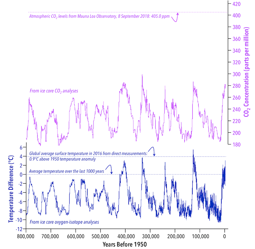
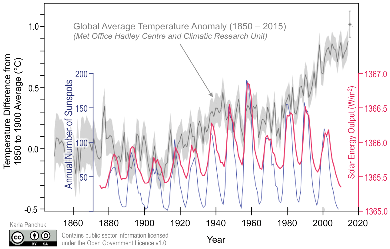
. [Learn more about PAGES2K and find data.](https://thinkprogress.org/most-comprehensive-paleoclimate-reconstruction-confirms-hockey-stick-e7ce8c3a2384/)_](figures/16-earth-system-change/figure-16-35.png)
Figure 16.35: Global average temperature change for the last 1000 years. Blue- The original “hockey stick” diagram showing a reconstruction of northern hemisphere temperatures using tree rings as a proxy. Red- Direct temperature measurements. Green dots- Global temperature reconstruction using a wide range of direct measurements, historical records, and proxies (sediments, ice cores, tree rings, corals, stalagmites, pollen). The original hockey stick diagram was the focus of much controversy because it was the first evidence of anthropogenic climate change that could be understood by the general public. The PAGES2K project sought to bring vast quantities of data to establish once and for all whether a global signal of warming could be reliably discerned. The result was very similar to the original hockey stick. Source: Karla Panchuk (2018) CC BY-SA 4.0. Modified after Klaus Bittermann (2013) CC BY-SA 4.0 view source. Learn more about PAGES2K and find data.
16.5.4.2 Sea Level Change
As of April 2018, global sea level has risen approximately 28 cm since 1800. According to satellite data, the average rate of change since 1993 has been a rise of approximately 3 mm per year. Part of the rise is due to the expansion of seawater as it warms. Another part of the rise is from water added by melting glaciers and other year-round land-based snow and ice. Note that melting of sea ice—ice already floating in the ocean—does not contribute directly to sea-level rise because the ice is already floating in the ocean.
Based on how much melting has occurred thus far, sea levels are projected to rise to between 47 cm and 130 cm above 1880 levels (Figure 16.36). However, there is some uncertainty about how melting rates will respond to changes in the Earth system that result from climate change, such as changes in currents, or seawater beneath the leading edge of melting ice sheets warming the ice from beneath. With that uncertainty factored in, sea level rise could be as low as 33 cm above 1880 levels, or more than 2 m higher.
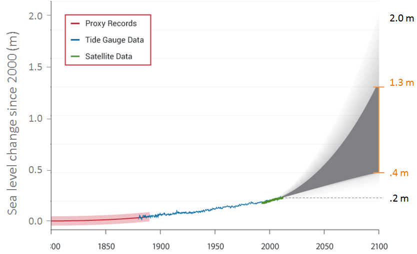 and J. Willis, Jet Propulsion Laboratory (2013). [View source and more information about this figure.](https://data.globalchange.gov/report/nca3/chapter/our-changing-climate/figure/past-and-projected-changes-in-global-sea-level-rise) Click the image for terms of use._](figures/16-earth-system-change/figure-16-36.png)
Figure 16.36: Measured and projected change in global average sea level. Data come from proxy records as well as from direct measurements from tidal gauges and satellite data. Projected sea level rise could be as little as 33 cm over 1800 levels, or as much as 206 cm. Source: Karla Panchuk (2018) modified after Steven Earle (2015) CC BY 4.0 view source and J. Willis, Jet Propulsion Laboratory (2013). View source and more information about this figure. Click the image for terms of use.
Keep in mind that the global average is indeed an average. Where ocean waters experience more warming, and thus more thermal expansion, sea level rise may be greater than elsewhere. Regions that are rebounding as ice melts could experience less sea level rise, or even a fall in sea level, because the elevation of the terrain is actually increasing over time. On the other hand, regions on the peripheral bulge around the margins of ice sheets could experience greater than average sea level rise because the terrain will subside at the same time that the oceans are gaining volume.
Areas that become flooded could experience greater than average sea level rise, because the weight of water causes the land to subside further. In the aftermath of Hurricane Harvey in September of 2017, measurements were reported that showed subsidence of up to 1.5 cm in the region of Houston, Texas. In this case, some of the subsidence could have been from sediments being compressed under the weight of flood waters, however the weight of water, like the weight of ice, does cause the crust to float lower in the mantle.
16.5.4.3 Melting Ice Sheets
Keeping track of how rapidly ice sheets are melting is important both for being able to predict future sea level change, and for knowing in general how rapidly the Earth system is changing. In a recent study, Bamber et al. (2018) analyzed satellite measurements to determine how much mass had been lost from the Antarctic ice sheets, the Greenland Ice Sheet, and from other glaciers and ice caps around the world since 1992 (Figure 16.37).
_](figures/16-earth-system-change/figure-16-37.jpg)
Figure 16.37: Large ice sheets of Antarctica and Greenland (blue) and glaciers and ice caps (yellow). Circles are proportional to the area of each region that is covered by glaciers. The green part of the circle indicates the proportion of the ice with margins resting on land, and the blue part indicates margins in the ocean. This difference is important in part because of the potential for faster melting when the base of an ice sheet is in contact with warming seawater. Source: Bamber et al. (2018) CC BY 4.0. View source (see Fig. 1)
The study found that over all, the mass of ice in ice sheets, ice caps, and glaciers has been falling at an increasing rate since 1992, and therefore adding to sea level at an increasing rate (Figure 16.38). The exception is the East Antarctic Ice Sheet, which actually showed an increase in mass during the studied interval. This is because snowfall has increased in the East Antarctic, to the point where more snow is falling now than at any time in the past 2000 years (Medley et al., 2017). The East Antarctic is warming just as the West is, but the difference is that the winds that preferentially bring precipitation to the East rather than the West can carry more moisture because the air is warmer.
_](figures/16-earth-system-change/figure-16-38.png)
Figure 16.38: Results of a study of the change in mass of ice on Earth’s surface. Satellite data show that over all, melting has accelerated since 1992. Source: Karla Panchuk (2018) CC BY 4.0, modified after Bamber et al. (2018) CC BY 4.0. View source (see Fig. 11)
16.6 Welcome to the Anthropocene
Geologists still have not agreed on an official start date for the Anthropocene Epoch, but it is unlikely that they would disagree that we are presently in it. What this means in practical terms is that humans today are experiencing the results of past human influence on the Earth system, and humans in the future will experience the results of decisions made today.
16.6.1 Data on Key Sources of Radiative Forcing
The Intergovernmental Panel on Climate Change (IPCC) was established by the United Nations in 1988 to help with those decisions. Is responsible for reviewing the scientific literature on climate change and issuing periodic reports on several topics, including the scientific basis for understanding climate change, our vulnerability to observed and predicted climate changes, and what we can do to limit climate change and minimize its impacts.
In their Fifth Assessment Report, Summary for Policy Makers, the IPCC identified the main contributions to heating or cooling our atmosphere, and the impact they had in 2011 compared to 1750, before the industrial age (Figure 16.39). The main natural source of radiative forcing is the sun, but it contributes relatively little compared to anthropogenic sources. The greatest contribution over all comes from anthropogenic CO2 (top row). Note that the bar sizes indicate the relative contribution, and correspond to the scale at the bottom of the diagram. Bars to the left of the zero line indicate cooling of the atmosphere, and bars to the right indicate warming. The column on the far right indicates how confident scientists are in their assessment of radiative forcing for each source (VH = very high; H = high; M = medium; L = low).
 Click the image for terms of use._](figures/16-earth-system-change/figure-16-39.jpg)
Figure 16.39: Anthropogenic and natural contributions to radiative forcing in 2011 compared to 1750. Source: IPCC (2013) View source (SPM.5, p. 14). Click the image for terms of use.
The biggest anthropogenic contributor to warming, CO2, accounts for 50% of positive forcing. CH4 and its atmospheric derivatives (CO2, H2O, and O3) account for 29%, and the halocarbon gases (mostly leaked from air-conditioning appliances) and nitrous oxide (N2O, from burning fossils fuels) account for 5% each. Carbon monoxide (CO, also produced by burning fossil fuels) accounts for 7%, and the volatile organic compounds other than methane (NMVOC) account for 3%.
CO2 emissions come mostly from coal- and gas-fired power stations, motorized vehicles (cars, trucks, and aircraft), and industrial operations (e.g., smelting), and indirectly from forestry. CH4 emissions come from production of fossil fuels (escape from coal mining and from gas and oil production), livestock farming (mostly beef), landfills, and wetland rice farming. N2O and CO come mostly from the combustion of fossil fuels. In summary, close to 70% of current anthropogenic GHG emissions come from fossil fuel production and use, while most of the rest comes from agriculture and landfills.
16.6.2 Projected Warming
The IPCC projects future warming by using scenarios that represent different possible paths that take into account global population, economic development, and global co-operation. In their best-case scenario, called RCP2.6 (RCP stands for representative concentration pathway, and 2.6 refers to a radiative forcing of 2.6 W/m2), global CO2 emissions begin to decline after 2020, and go to zero by 2080. Their worst-case scenario is RCP8.5, in which global CO2 emissions continue to rise rapidly. Intermediate scenarios reflect cases where global CO2 emissions eventually peak, but do not go to zero.
 Click the image for terms of use._](figures/16-earth-system-change/figure-16-40.png)
Figure 16.40: Model projections to 2100 for surface temperatures (a) and the extent of sea ice in September in the Northern Hemisphere (b). Black line: data; Grey shading: model attempts to simulate conditions from 1950 to 2005; Blue: best-case scenario with peak CO2 emissions in 2020 and zero emissions by 2080; Red: worst-case scenario with no decline in emissions. Numbers indicate the number of models run for each scenario. Shading indicates range of uncertainty. Source: IPCC (2013) View source (Fig. SPM.7, p. 14). Click the image for terms of use.
In the best-case scenario, temperatures stabilize at approximately 1 ºC above 1996 temperatures by the end of the century. As of 2018 there is no global plan in place that will meet the timeline of RCP2.6, and cause emissions to decline after 2020. For sea ice, all but the best-case scenario have the average sea ice extent beneath the dashed line, which effectively means the northern hemisphere would be ice-free.
16.6.3 Extreme Climate-System Events
In 2015 the World Meteorological Organization (WMO) published an analysis of extreme climate-system events, and showed that the number of such events globally was almost 5 times higher in the decade 2001-2010 than in the decade 1971-1980 (Figure 16.41).
 Click the image for terms of use._](figures/16-earth-system-change/figure-16-41.png)
Figure 16.41: Numbers of climate-system disasters between 1971 and 2010. Source: WMO (2015) Atlas of Mortality and Economic Losses from Weather, Climate and Water Extremes: 1970-2012. View source (p. 9). Click the image for terms of use.
Analyses of natural disasters and extreme weather events by the European Academies’ Science Advisory Council (EASAC) showed that from 1980 to 2010, extreme weather, floods, and mass movement related to floods increased by more than three-fold in Europe. In the same study, analyses of insurance-industry data showed that globally, Europe and South America are the least affected. The number of events has been more than twice as great in Asia, Australia/Oceania, and North America (EASAC, 2013). The EASAC recently published an updat to their study, to include data up to 2016. They now say that floods and mass movement events have increased in Europe by more than 4 times from 1980 levels (EASAC, 2018).
16.6.3.1 Extreme Temperatures
The major types of disasters reported by the WMO report are related to climate are floods and storms, but the health implications of extreme temperatures are also becoming a great concern. In the decade 1971 to 1980, extreme temperatures were the fifth most common natural disasters; by 2001 to 2010, they were the third most common.
For several weeks in July and August of 2010, a massive heat wave affected western Russia, especially the area southeast of Moscow. Temperatures soared to over 40°C, as much as 12°C above normal over a wide area, and wildfires raged in many parts of the country. Over 55,000 deaths are attributed to the heat and to respiratory problems associated with the fires (Figure 16.42).
_](figures/16-earth-system-change/figure-16-42.png)
Figure 16.42: Temperature anomalies across Russia and neighbouring regions during July 2010. Source: Earth Observatory (2010) Public Domain view source
A clue to explaining the heatwave was simultaneous flooding in Pakistan: in July, rainfalls were 70% higher than normal, and in August rainfalls were 102% above normal. Flooding from heavy rains combined with a burst dam impacted 18 million people, killing 1,985. These events were linked by a change in atmospheric circulation that caused weather patterns to stall out over Russia and Pakistan. The change itself was due in part to a decrease in the temperature differences between high and low latitudes, caused by warming in the north.
16.6.4 Sea-Level Rise and Tropical Storm Impacts
Projections for sea-level rise to the end of this century vary widely (Figure 16.36), however it is already the case that low-lying coastal regions are experiencing increased flooding during storm events. Flood defenses designed decades ago are or will soon be insufficient in the face of increasingly frequent and more extreme storm events. In a 2008 report, the Organisation for Economic Co-operation and Development (OECD) estimated that by 2070 approximately 150 million people living in coastal areas could be at risk of flooding due to the combined effects of sea-level rise, increased storm intensity, and land subsidence. The assets at risk (buildings, roads, bridges, ports, etc.) are on the order of $35 trillion ($35,000,000,000,000). Countries with the greatest exposure of population to flooding are China, India, Bangladesh, Vietnam, U.S.A., Japan, and Thailand. Some of the major cities at risk include Shanghai, Guangzhou, Mumbai, Kolkata, Dhaka, Ho Chi Minh City, Tokyo, Miami, and New York.
One of the other risks for coastal populations, besides sea-level rise, is that climate warming is also associated with an increase in the intensity of tropical storms (e.g., hurricanes or typhoons), which almost always bring serious flooding from intense rain and storm surges. It is difficult for climatologists to ascribe all of the characteristics of a particular tropical storm to climate change, but it is much easier to make a case for why tropical storms in general would become stronger, and have more of an impact on coastal regions.
When Hurricane Sandy hit New Jersey and New York in 2012 (Figure 16.43), it had a devastating impact in part because it smashed into the coast directly rather than moving parallel to the coast. There was some speculation that the unusual path was the result of changes in atmospheric circulation that were related to climate change. We can’t say for certain whether climate change caused Sandy to move the way it did, but we can say with confidence that climate change worsened the impact of Sandy through sea-level rise. Consider that, over the previous 100 years, sea level had risen a foot at the southern-most tip of Manhattan Island. The island was hit by a 14-foot storm-surge, higher than it would have been without sea-level rise.
_](figures/16-earth-system-change/figure-16-43.jpg)
Figure 16.43: Damage from Hurricane Sandy on the coast of New Jersey. Source: Master Sgt. Mark C. Olsen, New Jersey National Guard (2010) Public Domain view source
16.6.4.1 Tropical Storm Intensity
Tropical storms get their energy from the evaporation of warm seawater in tropical regions. In the Atlantic Ocean, this takes place between 8° and 20° N in the summer. A correlation has been observed between variations in the sea-surface temperature (SST) of the tropical Atlantic Ocean (Figure 16.44, red) and the amount of power represented by Atlantic hurricanes between 1950 and 2008 (blue). Not only has the overall intensity of Atlantic hurricanes increased with the warming since 1975, but the correlation between hurricanes and sea-surface temperatures is very strong over that time period.
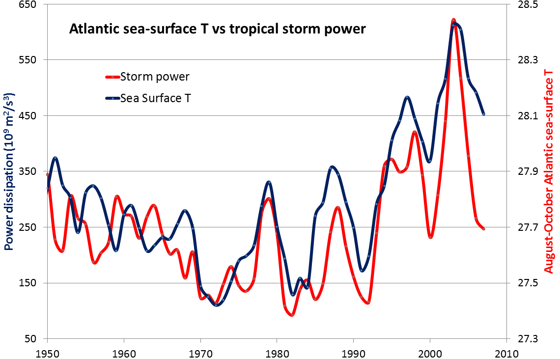/ [view data source](http://wind.mit.edu/~emanuel/Papers_data_graphics.htm) _](figures/16-earth-system-change/figure-16-44.png)
Figure 16.44: Relationship between Atlantic tropical storm cumulative annual intensity and Atlantic sea-surface temperatures. Source: Steven Earle (2015) CC BY 4.0 view source/ view data source
Because warm air is able to hold more water than cold air, the general global trend over the past century has been one of increasing precipitation (Figure 16.45). Note that this does not mean that precipitation has increased everywhere in the world. It means that even taking into account regions that have become drier, there is still more precipitation over all.
_](figures/16-earth-system-change/figure-16-45.png)
Figure 16.45: Global precipitation from 1901 to 2000. Source: Karla Panchuk (2018) CC BY 4.0, with data from NASA/GISS. Get data
16.6.5 Thawing Permafrost
Most of northern Canada has a layer of permafrost that ranges from a few centimetres to hundreds of metres in thickness. The same is true in Alaska, Russia, and Scandinavia. One problem that northern communities are currently dealing with is that thawing permafrost is weakening sediments that were previously solid and stable. This can cause structures to settle, or even to sustain serious damage. Another problem with the weakening that occurs when permafrost thaws is that mass wasting can occur (Figure 16.46). This is particularly dangerous for northern communities along coastlines, where homes may be near the shore and the slopes beneath them further weakened by strong wave action during severe storms.
_](figures/16-earth-system-change/figure-16-46.jpg)
Figure 16.46: A degrading permafrost site on the north coast of Alaska. Source: Alaska Science Center, U. S. Geological Survey (2016) Public Domain view source
A longer-term issue with thawing permafrost is that micro-organisms begin to decompose organic matter within the newly thawed sediments, releasing CO2 and CH4. The amount of these greenhouse gases released by decomposing organic matter could be enough to generate a significant positive feedback, accelerating warming further. In some polar regions, including northern Canada, permafrost also includes methane hydrate, a highly concentrated form of CH4 trapped in solid form. Breakdown of permafrost releases this CH4 as well.
16.6.6 Pests and Disease
The geographical ranges of diseases and pests, especially those caused or transmitted by insects, have been shown to extend toward temperate regions because of climate change. West Nile virus and Lyme disease are two examples that already directly affect Canadians, while dengue fever could be an issue in the future. Canadians are also indirectly affected by the increase in populations of pests such as the mountain pine beetle (Figure 16.47).
_](figures/16-earth-system-change/figure-16-47.jpg)
Figure 16.47: Mountain pine beetle damage in Manning Park, British Columbia. Source: Jonhall (2010) CC BY 3.0 view source
16.6.6.0.0.1 References
Berwyn, B. (2017, 27 March). Climate Change-Fueled Jet Stream Linked to Brutal Floods and Heatwaves, Says Study. View at Inside Climate News
Charley, S. (2013, 13 June). Hurricane Sandy took highly unusual path, but climate change doesn’t get the blame – yet. View at GeoSpace
European Academies’ Science Advisory Council. (2013). Trends in Extreme Weather Events in Europe: Implications for National and European Union Adaptation Strategies. Halle (Saale), Germany: German National Academy of Sciences. Full text
European Academies’ Science Advisory Council. (2018). Extreme weather events in Europe. Preparing for climate change adaptation: An update on EASAC’s 2013 study. Halle (Saale), Germany: German National Academy of Sciences. Full text
Furphy, D. (2013, 28 September). What on earth is an RCP? A quick guide to carbon dioxide emissions scenarios used by the IPCC Assessment Report 5. View at Medium
Intergovernmental Panel on Climate Change. (2013). _Summary for Policymakers. In: Climate Change 2013: The Physical Science Basis. __Contribution of Working Group I to the Fifth Assessment Report of the Intergovernmental Panel on Climate Change _[Stocker,T.F., D. Qin, G.-K. Plattner, M. Tignor, S.K. Allen, J. Boschung, A. Nauels, Y. Xia, V. Bex and P.M. Midgley (eds.)]. Cambridge University Press, Cambridge, United Kingdom and New York, NY, USA. Full text
Scott, M. (2011, 6 April). Heavy Rains and Dry Lands Don’t Mix: Reflections on the 2010 Pakistan Flood. View at Earth Observatory
World Meteorological Organization. (2014). Atlas of Mortality and Economic Losses from Weather, Climate, and Water Extremes (1970-2012). Geneva, Switzerland: World Meteorological Association. Full text
16.7 Summary
The topics covered in this chapter can be summarized as follows:
16.7.1 What Is the Earth System?
Viewing Earth as a system allows us to take into account the complex ways in which the atmosphere, hydrosphere, biosphere, and lithosphere interact. Positive feedbacks amplify changes in the Earth system, and negative feedbacks reduce them. The stability of the Earth system will depend on what feedbacks are available. The presence of ice sheets makes the Earth system less stable.
16.7.2 Causes of Climate Change
Weather describes day-to-day conditions, but climate refers to the long-term average conditions over decades or longer. Climate forcings alter climate. They include processes that change the rate and location of solar energy reaching Earth’s surface; processes that alter how ocean currents move heat around Earth’s surface; and processes that affect how heat moves into and out of the atmosphere. Climate forcings operate on a range of timescales, from billions of years to less than a decade. Changes in greenhouse gas concentrations and albedo are two climate forcings affected by human activities.
16.7.3 Methods for Studying Past Climate
Climate conditions for some of human history can be determined from direct measurements that have been recorded, but for studying paleoclimate it is often necessary to use proxy data. Proxy data come from natural materials that behave in a systematic way in response to climate conditions like temperature or precipitation. Proxies include tree ring data, stable isotopes, measurements of gas bubbles trapped in ice, and the geographic distribution of rocks and fossils.
16.7.4 Computer Models of the Earth System
Earth-system models use mathematical equations to simulate Earth-system processes. Models are set up and checked using real-life measurements. Model uncertainty is a number that tells us the likelihood that a particular model result falls within a certain range of values. It is a way to evaluate whether results can be used to draw meaningful conclusions.
16.7.5 Humans in the Earth System
Data show recognizable anthropogenic influence on the Earth system beginning when humans began to use fossil fuels for industrial purposes. CO2 in the atmosphere has the isotopic fingerprints of fossil fuels. The flow of anthropogenic carbon into the Earth system is relatively small compared to some natural flows, but natural processes do not remove all of what humans put in, causing CO2 to accumulate in the atmosphere.
16.7.6 Welcome to the Anthropocene
Humans today are experiencing the results of past human influence on the Earth system, and humans in the future will experience the results of decisions made today. The main source of radiative forcing is anthropogenic CO2. Humans are already experiencing extreme climate events related to warming. The best-case projected warming scenario will stabilize global average temperatures at ~1ºC above 1996 temperatures by the end of the century, but this will require a peak in anthropogenic CO2 emissions by 2020, and an end to anthropogenic CO2 emissions by 2080.
16.8 Chapter Review Questions
If you receive positive feedback on a project, this means someone says you did a good job. Does this mean a positive feedback in the climate system is also something good? Explain.
Why does the presence of ice sheets cause the Earth system to be less stable?
Using the orbital information on eccentricity, tilt, and precession, we could calculate variations in insolation for any latitude on Earth and for any month of the year. Why do we focus on a latitude of 65° N?
Explain how the positioning of Gondwana at the South Pole contributed to glaciation during the Paleozoic.
If the major currents in the oceans were to slow down or stop, how would that affect the distribution of heat on Earth, and what effect might that have on glaciation?
Most volcanic eruptions lead to short-term cooling, but long-term sustained volcanism can lead to warming. Describe the mechanisms for these two different consequences.
What property of greenhouse gases allows them to absorb infrared radiation and thus trap heat within the atmosphere?
What are the advantages of proxy data over direct measurements of climate? What are the disadvantages of using proxy data?
What are some steps that scientists take to help ensure that meaningful conclusions can be drawn from Earth-system computer models?
What evidence tells us that rising atmospheric CO2 levels are primarily the result of humans burning fossil fuels?
The flows of carbon through the carbon cycle that are related to human activities are actually much smaller than some natural flows. Why do human activities have such a large impact on the carbon cycle?
Some people argue that climate has always changed, and present-day climate change is not significant compared to the long-term record of Earth’s climate. Is it true that present-day climate signals show that changes are not significant compared to Earth’s long-term climate history? Explain your answer.
What climate mechanism links both extreme heat waves and droughts, and extreme flooding and rainfall events to climate change?
What evidence suggests that increasingly intense tropical storms can be expected as climate warms?
What are the potential impacts of thawing permafrost?
16.9 Answers to Chapter Review Questions
A positive feedback does not mean that something good is happening in the Earth system. Rather, it means that a change is being amplified by other Earth-system processes that were triggered by the change. From a human perspective, having a change amplified could be good or bad.
When ice is present, relatively small changes in temperature can trigger albedo feedbacks that amplify the change. If no ice is present, a small increase in temperature might not have much of an impact. But if ice is present, that small increase could be enough to cause the ice to melt, and decrease Earth’s albedo. If ice is created when the climate cools, further cooling can be triggered if the ice increases Earth’s albedo significantly.
We use 65° for estimating the glaciation potential of orbital variations because glaciers are most likely to form at high latitudes, where temperatures are cooler, and insolation less direct. We use 65° N rather than 65° S because for more than 50 million years the continents have been concentrated in the northern hemisphere. We use July instead of January, because for ice to form and remain year-round, it is necessary to have cool summers.
Gondwana was situated over the south pole for much of the Paleozoic. Not only was the land subject to temperatures cooler over all, and less direct insolation for part of the year, but the large size of the continent limited the extent to which heat from the ocean could reach the interior of the continent. The development of ice on Gondwana further cooled the planet through albedo feedback.
If the major currents in the oceans were to slow down or stop, the tropics would get hotter and the high-latitude areas would get colder, leading to expansion of glaciers and sea ice. The various feedbacks (e.g., higher albedo because of increased ice cover) would result in a cooler climate over all.
From a climate perspective, the two important volcanic gases are SO2 and CO2. SO2 is converted to aerosols which block sunlight and can lead to short-term cooling (lasting years). CO2 can lead to warming, but only in situations where there is an elevated level of volcanism over the long term.
Greenhouse gases vibrate at frequencies that are similar to those of infrared radiation. When infrared radiation hits a greenhouse gas molecule, the molecule’s vibrational energy is enhanced and the radiation energy is converted into heat, which is trapped within the atmosphere.
Proxy data can provide information about climate in the distant past, for times during which there were no direct measurements. As new techniques are developed, analyses of proxy data can improve, whereas direct measurements will have experimental errors related to the instruments used to make them at the time. A disadvantage of proxy data is that we don’t always have a detailed timeline to go with the data, and may need to rely on other lines of evidence to understand when the proxy data should apply. Special equipment or techniques may be needed to get proxy data from geological materials. It is also necessary to ensure that geological processes have not altered the materials in some way that makes the results of analyses unreliable.
Real-life measurements are used to set up the model, and to test that it can provide realistic results. Many different models may be used to study the same scenario, and the results compared. This helps scientists to compare the results of representing the Earth system in different ways. An estimate of uncertainty is provided so scientists can decide whether or not the range of uncertainty is too big, given the size of the Earth-system change being studied.
Data from ice cores and direct measurements show that atmospheric CO2 levels began to rise very rapidly at the same time that humans began using fossil fuels extensively to power activities like manufacturing and transportation. At the same time, the stable carbon-isotope composition of atmospheric CO2 began to decrease at a rate that is consistent with the stable carbon-isotope fingerprint of plant-derived organic matter. Also simultaneously, the radiocarbon age of atmospheric CO2 began to fall, consistent with carbon from very ancient plant sources being added to the atmosphere. Aside from the timing of geochemical changes matching the onset of the industrial era, there are no other sources of carbon that can account for the geochemical fingerprint in the atmosphere.
The reason that relatively small anthropogenic flows of carbon into the carbon cycle can have a big impact is that they aren’t being balanced by natural processes that can remove the extra carbon. The result is that carbon from anthropogenic activities is accumulating in the atmosphere and ocean.
In the past, Earth’s climate has been both much colder and much hotter than today. However, present day temperatures are significantly different compared to global average temperatures over the past 1000 years, and stand out in the data from the past 800,000 years. Atmospheric CO2 levels are much higher than at any time during the past 800,000 years, and on that timescale, the increase is almost instantaneous. Therefore, the magnitude of present-day change in the Earth-system stands out clearly from background conditions predating the appearance of anatomically modern humans. It is also happening much faster than even the most rapid carbon-release event that we know of in the rock record.
Climate warming happens more rapidly at high latitudes more than low latitudes, decreasing the temperature difference between them. The decreased difference allows atmospheric circulation patterns to “stall out” over a location for longer than usual. What would normally be a short heatwave lasts much longer, and a precipitation event that would normally move elsewhere after a short time is now halted in place for weeks.
See Figure 16.44. The power of tropical storms depends on the warmth of seawater. Data show that during particularly warm intervals, tropical storms are stronger. Data also show that the strength of storms over all is increasing as sea surface temperatures rise over time.
Frozen soils provide a solid foundation for buildings in northern communities. Melting of permafrost means the soil beneath buildings is weakened, and buildings can suffer structural damage. Thawing means that hillsides are more prone to mass wasting, especially terrain along coasts. In terms of the climate system, thawing of permafrost allows micro-organisms to decompose organic matter within previously-frozen sediments, releasing additional CO2 and CH4, and contributing to a positive feedback.
16.10 References
Caesar, I., Rahmstorf, S., Robinson, A., Feulner, G., & Saba, V. (2018). Observed fingerprint of a weakening Atlantic Ocean overturning circulation. _Nature 556. _194-196. https://doi.org/10.1038/s41586-018-0006-5 View abstract
Ingleby, B., & Huddleston, M. (2007). Quality control of ocean temperature and salinity profiles—Historical and real-time data. _Journal of Marine Systems, 65, _158-175. doi:10.1016/j.jmarsys.2005.11.019 Full text
Jouzel, J., Masson-Delmotte, V., Cattani, O., Dreyfus, G., Falourd, S., Hoffmann, G., Minster, B., Nouet, J., Barnola, J.M., Chappellaz, J.A., Fischer, H., Gallet, J.C., Johnsen, S.J., Leuenberger, M., Loulergue, L., Luethi, D., Oerter, H., Parrenin, F., Raisbeck, G.M., Raynaud, D., Schilt, A., Schwander, J., Selmo, E., Souchez, R., Spahni, R., Stauffer, B., Steffensen, J.P., Stenni, B., Stocker, T.F., Tison, J.L., Werner, M., & Wolff, E.W. (2007). Orbital and Millennial Antarctic Climate Variability over the Past 800,000 Years. Science 317(5839), 793-797. Get data
Lüthi, D., Le Floch, M., Bereiter, B.; Blunier, T., Barnola, J.M., Siegenthaler, U., Raynaud, D., Jouzel, J., Fischer, H., Kawamura, K., & Stocker, T.F. (2008). High-resolution carbon dioxide concentration record 650,000-800,000 years before present. Nature (453), 379-382. Get data
Met Office Hadley Centre (n.d.) EN3: quality controlled subsurface ocean temperature and salinity data. Visit website (data available). Note: EN4 data set (new version) available here.
RAPID-AMOC (n.d.) RAPID: monitoring the Atlantic Meridional Overturning Circulation at 26.5°N since 2004. Visit website (data available)
Robson, J., Hodson, D., Hawkins, E., & Sutton, R. (2014). Atlantic overturning in decline? Nature Geoscience 7(2-3). https://doi.org/10.1038/ngeo2050 Open access version
Shaffrey, L.C., Stevens, I., Norton, W. A., Roberts, M. J., Vidale, P. L., Harle, J. D., Jrrar, A., Stevens, D. P., Woodage, M. J., Demory, M. E., Donners, J., Clark, D. B., Clayton, A., Cole, J. W., Wilson, S. S., Connelley, W. M., Davies, T. M., Iwi, A. M., Johns, T. C., King, J. D., New, A. L., Singlo, J. M., Slingo, A., Steenman-Clark, L., & Martin, G. M. (2009). U.K. HiGEM: The New U.K. High-Resolution Global Environment Model—Model Description and Basic Evaluation. Journal of Climate 22, 1861 - 1896. doi:10.1175/2008JCLI2508.1 Full text
Smith, D. M., & Murphy, J. M. (2007). An objective ocean temperature and salinity analysis using covariances from a global climate model. Journal of Geophysical Research, 112(C02022). doi:10.1029/2005JC003172
Thornalley, D. J. R., Oppo, D. W., Ortega, P., Robson, J. I., Brierley, C. M., Davis, R., Hall, I. R., Moffa-Sanchez, P., Rose, N. L., Spooner, P. T., Yashayaev, I., & Keigwin, L. D. (2018). Anomalously weak Labrador Sea convection and Atlantic overturning during the past 150 years. _Nature 556, _227-230. https://doi.org/10.1038/s41586-018-0007-4 View abstract
Ridge, J.C. (2008) The North American Glacial Varve Project. Retrieved from http://eos.tufts.edu/varves
Zhang, J., & Crowley, T. (1989). Historical Climate Records in China and Reconstruction of Past Climates. Journal of Climate 2(8), 833-849. https://doi.org/10.1175/1520-0442(1989)002<0833:HCRICA>2.0.CO;2 Full text
Simons, T. J., & Schertzer, W. M. (1989) The circulation of Lake Ontario during the summer of 1982 and the winter of 1982/83. Burlington, ON: Environment Canada. Full text
Slingerland, R., & Kump, L. (2011). _Mathematical Modeling of Earth’s Dynamical Systems__: __A Primer_. Princeton, NJ: Princeton University Press.
Bajželj, B., Allwood, J. M., and Cullen, J. M. (2013). Designing Climate Change Mitigation Plans That Add Up. Environmental Science & Technology 47, 8062-8069. doi: 10.1021/es400399h. Retrieved from http://pubs.acs.org/doi/pdf/10.1021/es400399h
Bamber, J. L., Westaway, R. M., Marzeion, B., & Wouters, B. (2018). The land ice contribution to sea level during the satellite era. Environmental Research Letters 13(2018). https://doi.org/10.1088/1748-9326/aac2f0 Full text
Böhm, F., Haase-Schramm, A., Eisenhauer, A., Dullo, W.-C., Joachimski, M. M., Lehnert, H., & Reitner, J. (2002). Evidence for preindustrial variations in the marine surface water carbonate system from coralline sponges. Geochem. Geophys. Geosyst., 3(3), 10.1029/2001GC000264. Retrieved from http://onlinelibrary.wiley.com/doi/10.1029/2001GC000264/epdf
Earth System Research Laboratory, Global Monitoring Division, NOAA (n.d.). The Data: What 14C Tells Us. Visit website
Fischedick M., Roy, J., Abdel-Aziz, A., Acquaye, A., Allwood, J. M., Ceron, J.-P., Y. Geng, Y., Kheshgi, H., Lanza, A., Perczyk, D., Price, L., Santalla, E., Sheinbaum, C., and Tanaka, K. (2014). Industry. In: Climate Change 2014: Mitigation of Climate Change. Contribution of Working Group III to the Fifth Assessment Report of the Intergovernmental Panel on Climate Change. Edenhofer, O., Pichs-Madruga, R., Sokona, Y., Farahani, E., Kadner, S., Seyboth, K., Adler, A., Baum, I., Brunner, S., Eickemeier, P., Kriemann, B., Savolainen, J., Schlömer, S., von Stechow, C., Zwickel, T., and Minx, J. C. (eds.). Cambridge University Press, Cambridge, United Kingdom and New York, NY, USA. Retrieved from https://www.ipcc.ch/pdf/assessment-report/ar5/wg3/ipcc_wg3_ar5_chapter10.pdf
Madrigal, A. C. (2017, September 5) The Houston Flooding Pushed the Earth’s Crust Down 2 Centimeters. View at The Atlantic.
Medley, B., McConnell, J. R., Neumann, T. A., Reijmer, C. H., Chellman, N., Sigl, M., & Kipfstuhl, S. (2018). Temperature and Snowfall in Western Queen Maud Land Increasing Faster Than Climate Model Projections. Geophysical Research Letters 45(3), 1472-1480.https://doi.org/10.1002/2017GL075992
Rahmstorf, S. (2013). Most Comprehensive Paleoclimate Reconstruction Confirms Hockey Stick. View at ThinkProgress.org
Roser, M., & Ortiz-Ospina E. (2018). World Population Growth. View at OurWorldInData.com
Rubino, M., Etheridge, D. M., Trudinger, C. M., Allison, C. E., Battle, M. O., Langenfelds, R. L., Steele, L. P., Curran, M., Bender, M., White, J. W. C., Jenk, T. M., Blunier, T., & Francey, R. J. (2013). A revised 1000-year atmospheric δ13C‐CO2 record from Law Dome and South Pole, Antarctica. Journal of Geophysical Research: Atmospheres 118, 8482–8499. doi:10.1002/jgrd.50668 Full text