Chapter 14 Streams and Floods
Adapted from Physical Geology, First University of Saskatchewan Edition (Joyce M. McBeth) and Physical Geology (Steven Earle)
Learning Objectives
After reading this chapter, completing the exercises within it, and answering the questions at the end, you should be able to:
- Explain the hydrological cycle, its relevance to streams, and describe the residence time of water in these systems
- Describe what a drainage basin is, and explain the origins of the different types of drainage patterns
- Explain how streams become graded, and how certain geological and anthropogenic changes can result in a stream becoming ungraded
- Describe the formation of stream terraces
- Describe the processes that move sediments in streams, and how changes in stream velocity affect the types of sediments that are moved by the stream
- Explain the origin of natural stream levees
- Describe the process of stream evolution and the types of environments where one would expect to find straight-channel, braided, and meandering streams
- Describe the annual flow characteristics of typical streams in Canada and the processes that lead to flooding
- Describe some of the important historical floods in Canada
- Determine the probability of floods of various magnitudes, based on the flood history of a stream
- Explain some of the steps that we can take to limit damage from flooding
](figures/14-streams-and-floods/figure-14-1.jpg)
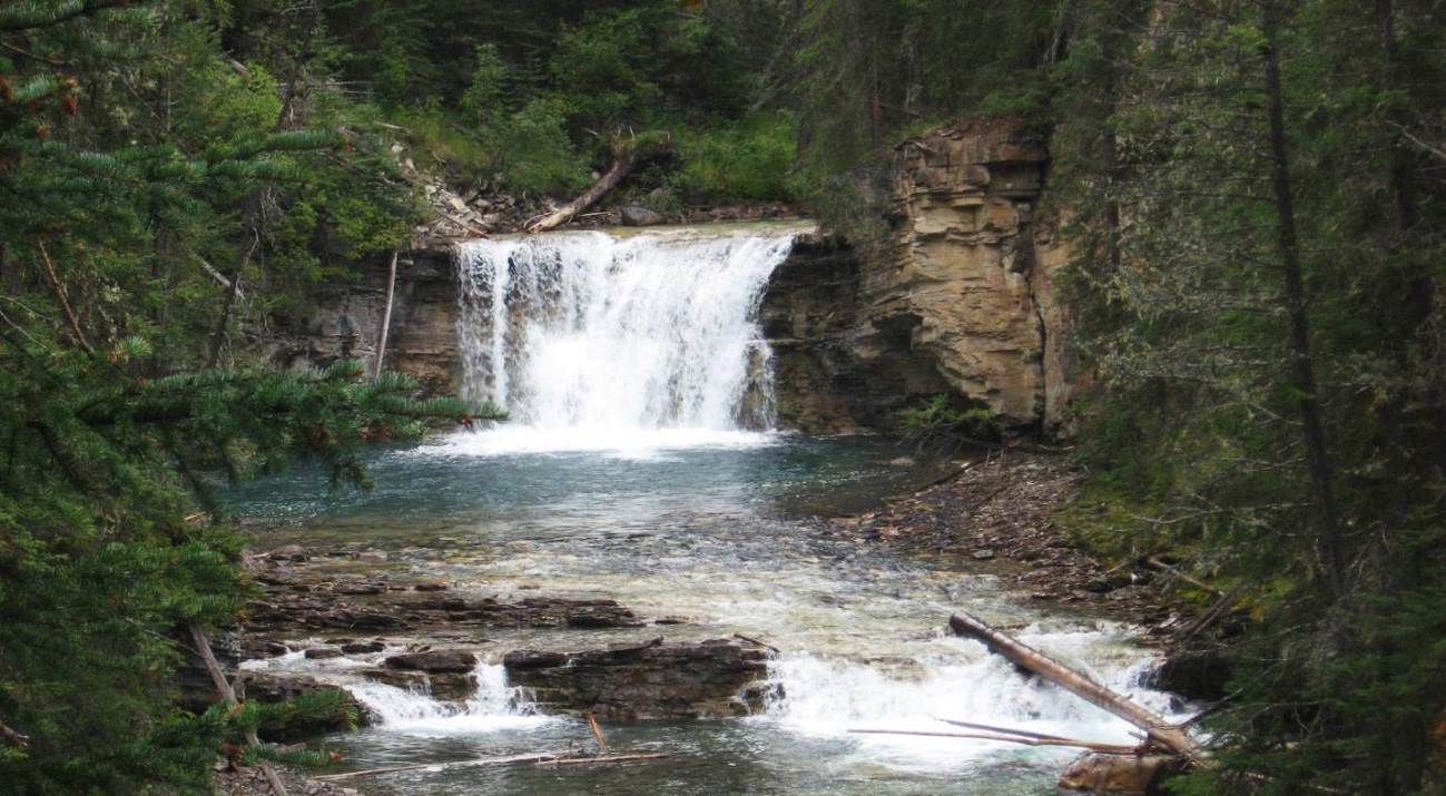
Figure 14.1: A small waterfall on Johnston Creek in Johnston Canyon, Banff National Park, AB Source: Steven Earle (2015) CC BY 4.0 view source
14.0.0.1 Why Study Streams?
Streams are the most important agents of erosion and transportation of sediments on Earth’s surface at this time in Earth’s history. They are responsible for generating much of the topography on that land surfaces that we see around us. They are places of beauty and tranquility, and they provide much of the water that is essential to our existence. But streams are not always peaceful and soothing. During large storms and rapid snowmelts, they can become raging torrents capable of moving cars and houses, and destroying roads and bridges. When they spill over their banks, they can flood huge areas, devastating populations and infrastructure. Over the past century, many of the most damaging natural disasters in Canada have been floods.
14.1 The Hydrological Cycle
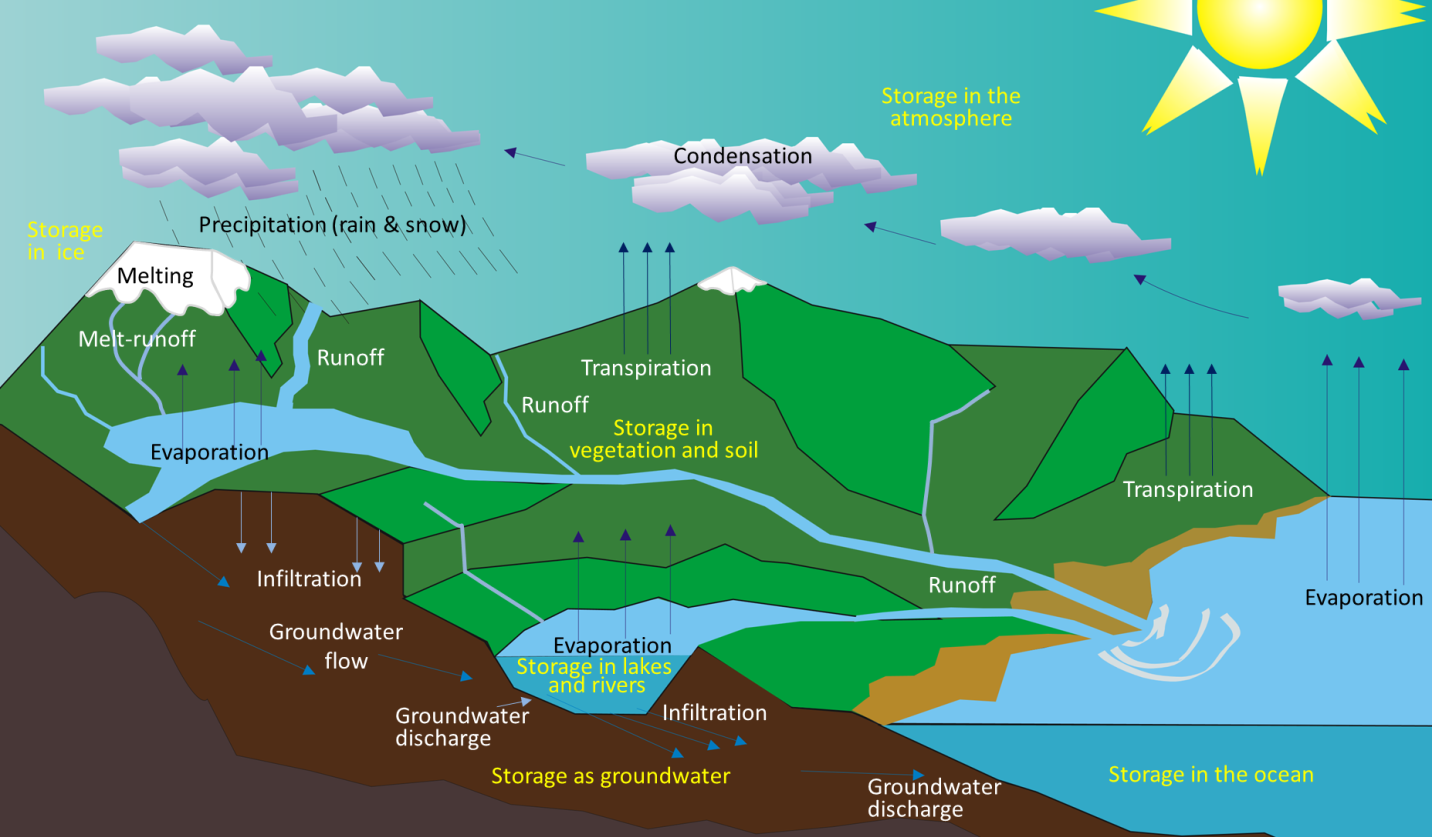
Water is constantly on the move. It is evaporated from the oceans, lakes, streams, the surface of the land, and from plants (transpiration) by solar energy (Figure 14.2). It is transported in its gaseous form through the atmosphere by the wind and condenses to form clouds of water droplets or ice crystals. It falls to the Earth’s surface as rain or snow and flows through streams, into lakes, and eventually back to the oceans. Water on the surface and in streams and lakes infiltrates the ground to become groundwater. Groundwater slowly moves through soils, surficial materials, and pores and cracks in the rock. The groundwater flow paths can intersect with the surface and the water can then move back into streams, lakes and oceans.
 after Wikimedia user "Ingwik" (2010) CC-BY-SA 3.0. [view source](https://commons.wikimedia.org/wiki/File:Water_cycle_blank.svg)](figures/14-streams-and-floods/figure-14-2.png)
Figure 14.2: The various components of the water cycle. Black or white text indicates the movement or transfer of water from one reservoir to another. Yellow text indicates the storage of water . Source: Steven Earle (2015) CC BY-SA 3.0 view source after Wikimedia user “Ingwik” (2010) CC-BY-SA 3.0. view source
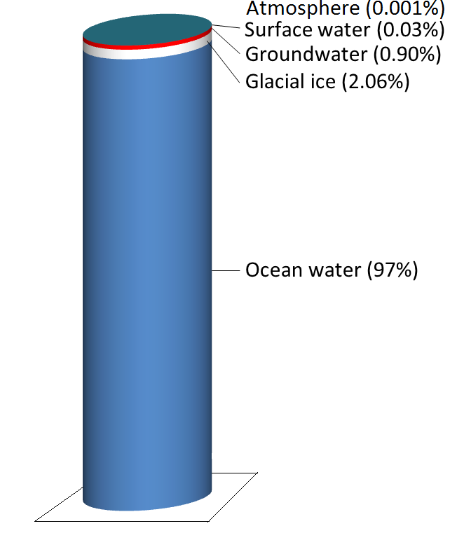
Water is stored in various reservoirs as it moves across and through the Earth. A reservoir is a space that stores water. It can be a space we can easily visualize (such as a lake) or a space that is more difficult to visualize (such as the atmosphere or the groundwater in a region). The largest reservoir is the ocean, accounting for 97% of the total volume of water on Earth (Figure 14.3). Ocean water is salty, but the remaining 3% of water on Earth is fresh water. Two-thirds of our fresh water is stored in the ground and one-third is stored in ice. The remaining fresh water (about 0.03% of the total) is stored in lakes, streams, vegetation, and the atmosphere.
, data from USGS Water Science School (2016) [view source](http://bit.ly/USGSH2O)](figures/14-streams-and-floods/figure-14-3.png)
Figure 14.3: The storage reservoirs for water on Earth. Glacial ice is represented by the white band, groundwater the red band, and surface water the very thin blue band at the top. The 0.001% stored in the atmosphere is not shown. Source: Steven Earle (2015) CC BY 4.0 view source, data from USGS Water Science School (2016) view source
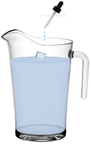
To put these percentages in perspective, we can compare a 1 litre container of water to the entirety of the Earth’s water supply (Figure 14.4). We start by almost filling the container with 970 ml of water and 34 g of salt, to simulate all the sea water on Earth. Then we add one regular-sized (ca 20 ml) ice cube (representing glacial ice) and two teaspoons (ca 10 ml) of groundwater. All of the water that we see around us in lakes and streams and in the atmosphere can be represented by adding three more drops of water from an eyedropper.
](figures/14-streams-and-floods/figure-14-4.png)
Figure 14.4: Representation of the Earth’s water in a 1 litre container. The three drops represent all of the fresh water in lakes, streams, and wetlands, plus all of the water in the atmosphere. Source: Steven Earle (2015) CC BY 4.0 view source
Although the water in the atmosphere is only a small proportion of the total water on Earth, the volume is still very large. At any given time, there is the equivalent of approximately 13,000 km3 of water in the air in the form of water vapour and water droplets in clouds. Water is evaporated from the oceans, vegetation, and lakes at a rate of 1,580 km3 per day, and each day nearly the same volume falls back as rain and snow over the oceans and land. Most of the precipitation that falls onto land returns to the ocean in the form of stream flow (117 km3/day) and groundwater flow (6 km3/day). Most of the rest of this chapter is about this 117 km3/day of streamflow.
14.1 Exercise 14.1 How Long Does Water Stay in the Atmosphere?
The residence time of a water molecule in the atmosphere (or any of the other reservoirs) can be estimated by dividing the total amount of water in the reservoir by the rate at which it is removed. For the atmosphere, we know that the reservoir size is 13,000 km3, and the rate is 1,580 km3/day. If we divide 13,000 km3 by 1,580 km3/day, we get 8.22 days. This means that, on average, a molecule of water stays in the atmosphere for just over eight days. “Average” needs to be emphasized here because some molecules remain in the air for only a few hours, while others may remain in the air for weeks.
The volume of the oceans is 1,338,000,000 km3 and the rate of removal of water from the oceans is approximately the same as the atmosphere (1,580 km3/day). What is the average residence time of a water molecule in the ocean?
14.2 Drainage Basins
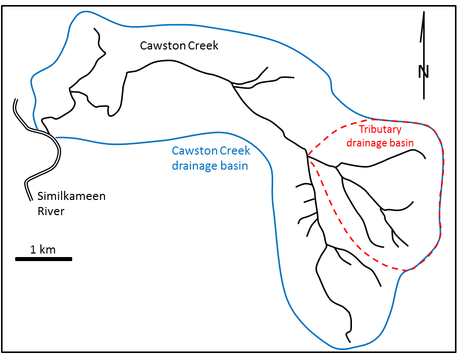
A stream is a body of flowing surface water of any size, ranging from a tiny trickle to a mighty river. The area from which the water flows to form a stream is known as its drainage basin or watershed. All of the precipitation (rain or snow) that falls within a drainage basin eventually flows into its stream, unless some of this water is able to cross into an adjacent drainage basin via groundwater flow. An example of a drainage basin is shown in Figure 14.5
](figures/14-streams-and-floods/figure-14-5.png)
Figure 14.5: A schematic diagram of the drainage basin of Cawston Creek near Keremeos, BC. The blue line shows the extent of the drainage basin. The dashed red line is the drainage basin of one of its tributaries. Source: Steven Earle (2015) CC BY 4.0 view source
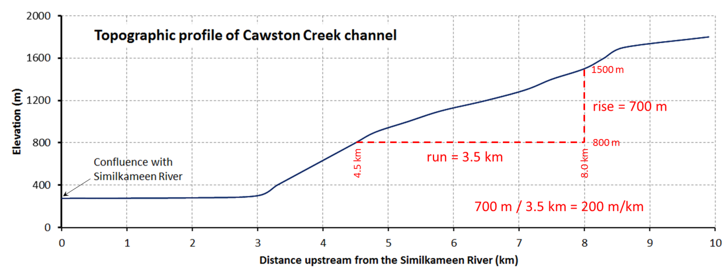
An important characteristic of streams is their gradient, the rate of change in elevation with distance along the stream. A steep gradient has a rapid change in elevation with horizontal distance, and a shallow gradient has a slow change in elevation with horizontal distance. Cawston Creek drainage basin in BC is approximately 25 km2 and is a typical small drainage basin within a very steep glaciated valley. As shown in Figure 14.6, the upper and middle parts of the creek have steep gradients averaging about 200 m/km but ranging from 100 to 350 m/km, and the lower part, within the valley of the Similkameen River, is relatively flat at <5 m/km.
The shape of the valley has changed through time to result in the shape we see now. First, there was tectonic uplift (related to tectonic plate convergence). Then the landscape changed due to stream erosion and mass wasting (landslides). This was followed by several episodes of glacial erosion. Finally, there was post-glacial stream erosion up to the present time. The lowest elevation of Cawston Creek (275 m, where the creek flows into the Similkameen River) is its base level. Cawston Creek cannot erode below this level unless the Similkameen River erodes deeper into its flood plain (the area that is inundated during a flood). Base level is the elevation where a stream will no longer erode deeper into the bedrock or sediments it flows through, because the elevation of the stream does not drop below this level, and further erosion can only occur if there is an elevation drop to propel the water deeper due to the force of gravity.
The ocean is the ultimate base level, but lakes and other rivers act as base levels for many smaller streams.
](figures/14-streams-and-floods/figure-14-6.png)
Figure 14.6: Profile of the main portion of Cawston Creek near Keremeos, BC. The maximum elevation of the drainage basin is about 1,840 m, near Mount Kobau. The base level is 275 m, at the Similkameen River. As shown, the gradient of the stream can be determined by dividing the change in elevation between any two points (rise) by the distance between those two points (run). Source: Steven Earle (2015) CC BY 4.0 view source
The water supply for the Vancouver, BC metropolitan area comes from three large drainage basins on the north shore of Burrard Inlet, as shown in Figure 14.7 This map illustrates the concept of a drainage basin divide. The boundary between two drainage basins is the ridge of land between them. A drop of rain falling on the boundary between the Capilano and Seymour drainage basins, for example, could flow into either basin. Rain falling on the Capilano basin side cannot flow into the Seymour drainage basin, because of the drainage basin divide.
](figures/14-streams-and-floods/figure-14-7.jpg)
Figure 14.7: The three drainage basins that supply water to the metropolitan Vancouver, BC area. Source: Wikimedia user “Alaidlaw” (2016) CC BY-SA 2.0. view source
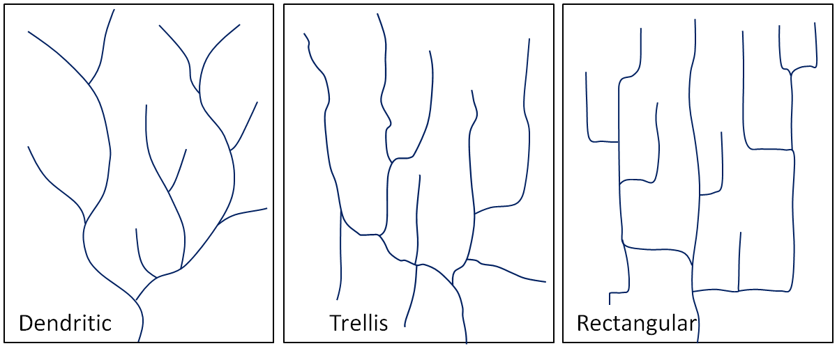
The pattern of tributaries within a drainage basin depends largely upon the type of underlying rock, and on structures within that rock such as folds, fractures, and faults. Three types of drainage patterns are illustrated in Figure 14.8 ____Dendritic__ patterns__, which are by far the most common, develop in areas where the rock (or unconsolidated material) beneath the stream does not have structures that control the stream flow patterns such as folds and joints; the materials can be eroded by the stream equally easily in all directions. Most areas of British Columbia have dendritic patterns, as do most areas of the prairies and the Canadian Shield.
____Trellis__ drainage__ patterns typically develop where sedimentary rocks have been folded or tilted, and then eroded to varying degrees depending on their resistance to erosion. The Rocky Mountains of BC and AB have some fine examples of trellis drainage.
Rectangular patterns develop in areas that have very little topography and a system of bedding planes, fractures, or faults that form a rectangular network. Rectangular drainage patterns are rare in Canada
](figures/14-streams-and-floods/figure-14-8.png)
Figure 14.8: Typical dendritic, trellis, and rectangular stream drainage patterns. Source: Steven Earle (2015) CC BY 4.0 view source
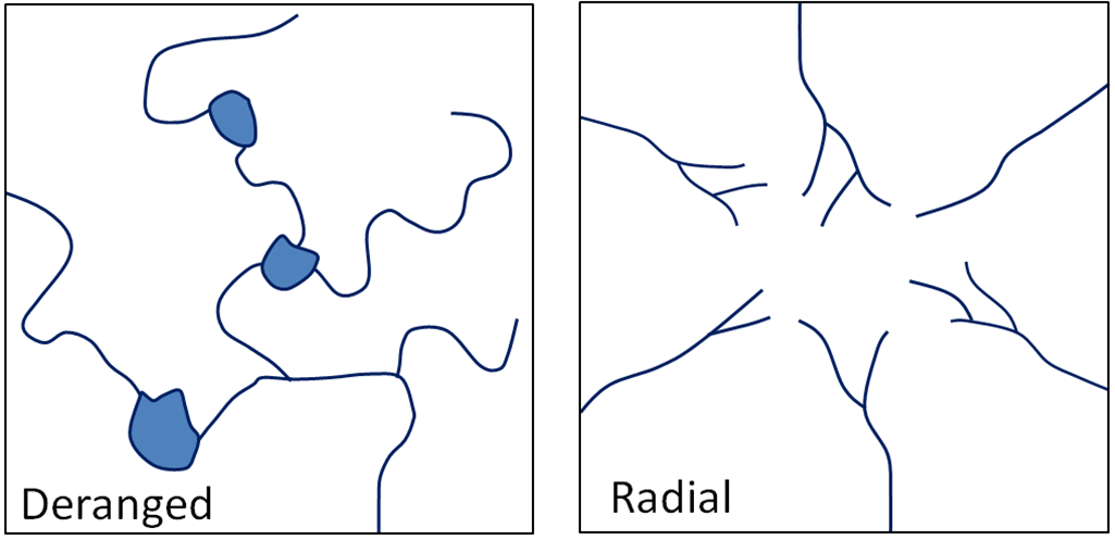
In many parts of Canada, especially relatively flat areas with thick glacial sediments, and throughout much of Canadian Shield in eastern and central Canada, drainage patterns are chaotic , also known as deranged (Figure 14.9, left). Lakes and wetlands are common in this type of environment.
__Radial __drainage (Figure 14.9, right) is a pattern that forms around isolated mountains (such as volcanoes) or hills. The individual streams that radiate out from the hill typically have dendritic drainage patterns.
](figures/14-streams-and-floods/figure-14-9.png)
Figure 14.9: Left: a typical deranged pattern; right: a typical radial drainage pattern developed around a mountain or hill. Source: Steven Earle (2015) CC BY 4.0 view source
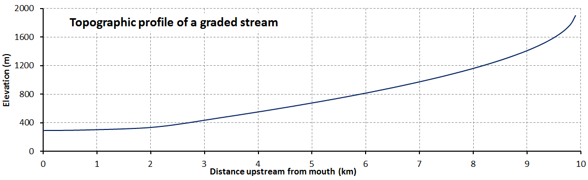
The process of a stream eroding downward into bedrock is called downcutting. Over geological time, and during tectonic quiescence, a stream will erode its drainage basin into a smooth profile similar to that shown in Figure 14.10 This is called a graded stream. Graded streams are steepest in their headwaters and their gradient gradually decreases toward their mouths. Ungraded streams are still in the process of rapidly eroding and downcutting their drainage basin, they have steep sections at various points, and typically have rapids and waterfalls at numerous locations along their lengths (e.g., Cawston Creek, Figure 14.6).
](figures/14-streams-and-floods/figure-14-10.png)
Figure 14.10: The topographic profile of a typical graded stream. Source: Steven Earle (2015) CC BY 4.0 view source
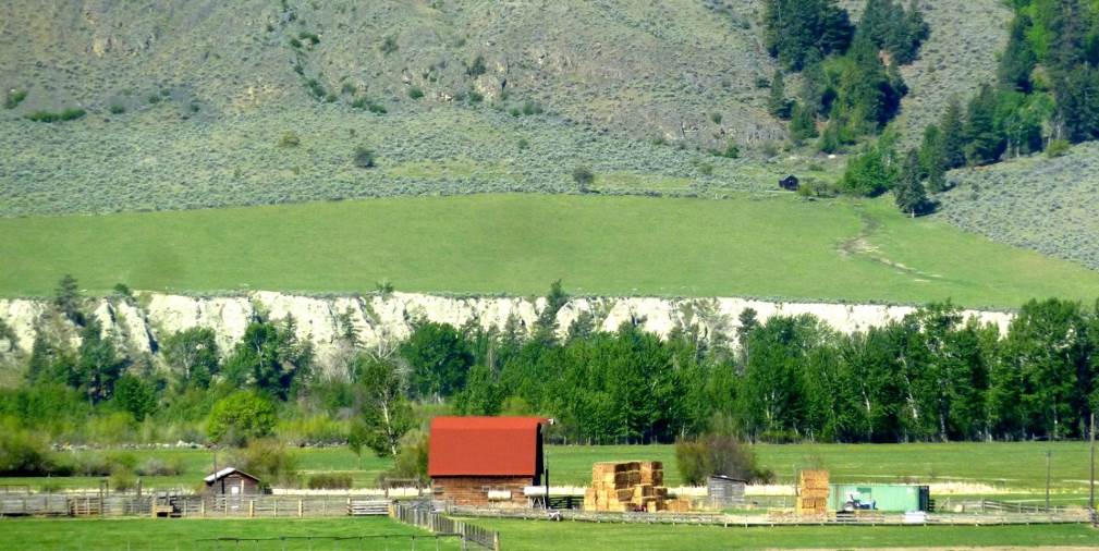
A graded stream can become ungraded if there is renewed tectonic uplift, or if there is a change in the base level. Base level changes can occur due to tectonic uplift or some other reason such as construction of a dam downstream. As stated earlier, the base level of Cawston Creek is defined by the level of the Similkameen River, but this can change, and has done so in the past. Figure 14.11 shows the valley of the Similkameen River in the Keremeos area. The river channel is just beyond the row of trees. The green field in the distance is underlain by material eroded from the hills behind and deposited by a small creek (not Cawston Creek) adjacent to the Similkameen River when its level was higher than it is now. Some time in the past several centuries, the Similkameen River eroded down through these deposits (forming the steep bank on the other side of the river), and the base level of the small creek was lowered by about 10 m. Over the next few centuries, this creek will erode through the sediments and eventually become graded again.
](figures/14-streams-and-floods/figure-14-11.jpg)
Figure 14.11: An example of a change in the base level of a small stream that flows into the Similkameen River near Keremeos. The previous base level was near the top of the sandy bank. The current base level is the Similkameen River, located on the far side of the line of trees. Source: Steven Earle (2015) CC BY 4.0 view source
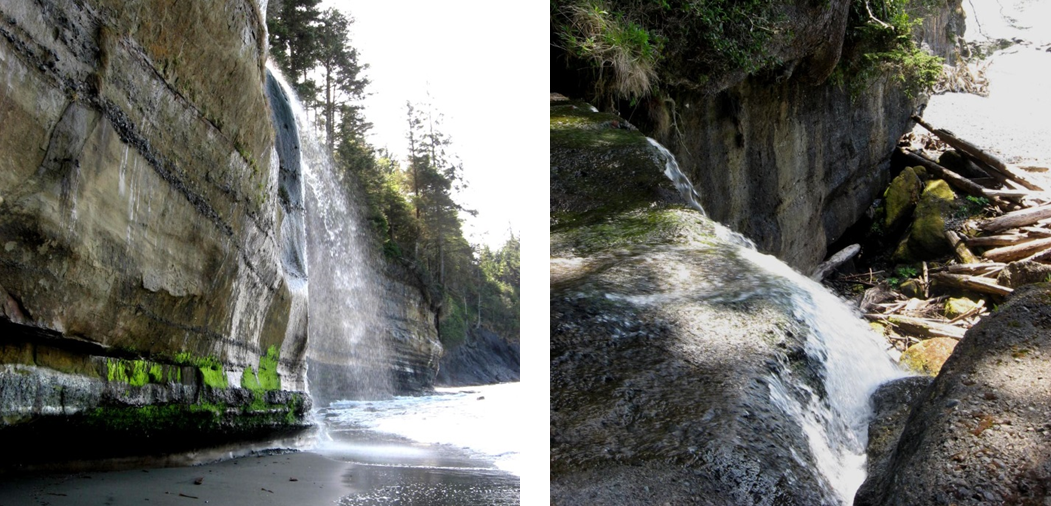
Another example of a change in base level can be seen along the Juan de Fuca Trail on southwestern Vancouver Island. As shown in Figure 14.12, many of the small streams along this part of the coast flow into the ocean as waterfalls. It is evident that the land in this area has risen by about 5 m in the past few thousand years, probably in response to deglaciation. The streams that used to flow directly into the ocean now have a lot of downcutting to do before they will be a graded stream again.
](figures/14-streams-and-floods/figure-14-12.png)
Figure 14.12: Two streams with a lowered base level on the Juan de Fuca Trail, southwestern Vancouver Island. Source: Steven Earle (2015) CC BY 4.0 view source
Sediments accumulate within the channel and flood plain of a stream, and then, if the base level changes, or if there is less sediment supplied to the stream to deposit, the stream may cut down through these existing sediments to form terraces. A terrace on the Similkameen River is shown in Figure 14.11 and terraces on the Fraser River are shown in Figure 14.13.
](figures/14-streams-and-floods/figure-14-13.jpg)
Figure 14.13: Terraces on the Fraser River north of Lillooet, BC (above the river on the left-hand side of the image). Source: Wikimedia user “China Crisis” (2007) CC BY-SA 3.0. view source
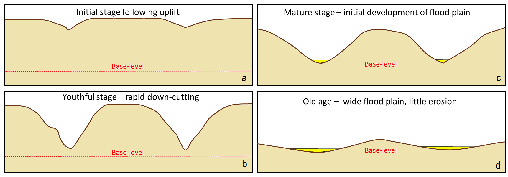
In the late 19th century, American geologist William Davis proposed that streams and the surrounding terrain develop in a cycle of erosion (Figure 14.14). Following tectonic uplift, the stream patterns are immature. Streams erode quickly, developing deep V-shaped valleys that tend to follow relatively straight paths. Gradients are high, and profiles are ungraded. Rapids and waterfalls are common. As the landscape matures, the streams erode wider valleys and deposited thick sediment layers. Even after maturity, gradients are slowly reduced and grading increases. In old age, streams are surrounded by rolling hills, and they occupy wide sediment-filled valleys. Meandering patterns are common, and erosion now is focussed towards the channel walls, with little downcutting.
](figures/14-streams-and-floods/figure-14-14.png)
Figure 14.14: A depiction of the Davis cycle of erosion: a: initial stage, b: youthful stage, c: mature stage, and d: old age . Source: Steven Earle (2015) CC BY 4.0 view source
Davis’s work was done long before the idea of plate tectonics, and he was also not familiar with the impacts of glacial erosion on streams and their environments. While some parts of his idea are out of date, it is still a useful way to understand streams and their evolution. Plate tectonic activity and other processes such as isostatic rebound after glaciation results in uplift that alters stream gradients, so streams are constantly adjusting due to these changing conditions. It would be relatively rare to find a stream that is able to mature through all of these stages without interruption.
14.2 Exercise 14.2 The Effect of a Dam on Base Level
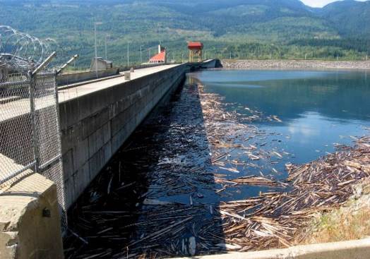 Revelstoke Dam and Revelstoke Lake on the Columbia River at Revelstoke, BC. Source: Steven Earle (2015) CC BY 4.0 [view source](https://opentextbc.ca/geology/wp-content/uploads/sites/110/2015/08/Revelstoke-Dam-and-Revelstoke-Lake.jpg)](https://openpress.usask.ca/app/uploads/sites/29/2017/05/Revelstoke-Dam-and-Revelstoke-Lake.jpg)
Figure 14.15: Revelstoke Dam and Revelstoke Lake on the Columbia River at Revelstoke, BC. Source: Steven Earle (2015) CC BY 4.0 view source
When a dam is built on a stream, a reservoir (artificial lake) forms behind the dam. The dam reservoir temporarily (for many decades at least) creates a new base level for the part of the stream above the reservoir. How does the formation of a dam reservoir affect the stream where it enters the reservoir, and what happens to the sediment it was carrying? The water leaving the dam has no sediment in it. Why? How does this affect the stream below the dam?
14.3 Stream Erosion and Deposition
14.3.1 Stream Velocity Depends on the Shape and Size of the Channel
Flowing water is a very important mechanism for both erosion and deposition. Water flow in a stream is primarily related to the stream’s gradient, but it is also controlled by the geometry of the stream channel. As shown in Figure 14.16, water flow velocity decreases due to friction along the stream bed. The stream is thus slowest at the bottom and edges and fastest near the surface and in the middle of the stream (where there is the least amount of friction). The velocity just below the surface of the water is typically a little higher than right at the surface because of friction between the water and the air. On a curved section of a stream, flow is fastest on the outside of the curve and slowest on the inside of the curve.
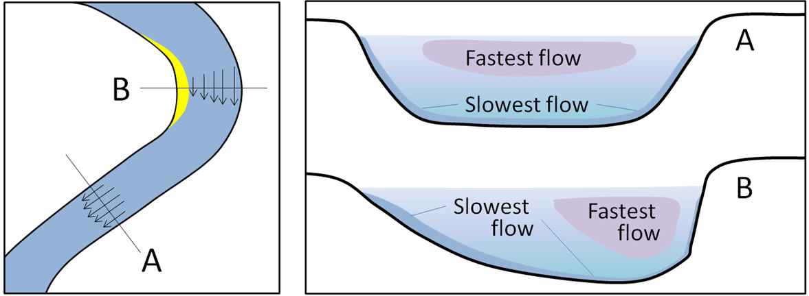](figures/14-streams-and-floods/figure-14-15.png)
Figure 14.16: The relative velocity of stream flow depending on whether the stream channel is straight or curved (left). (Right) it is also dependent on the water depth. The length of each of the arrows indicates the relative velocity of the stream at that position in the channel. Shorter arrows mean slower flow . Source: Steven Earle (2015) CC BY 4.0 view source
Another important factor influencing stream-water velocity is the ____discharge____, or volume of water passing a point in a unit of time (e.g., m3/second). Water levels rise during a flood and due to the higher discharge of water the stream flow velocity increases. The higher discharge also increases the cross-sectional area of the stream, so it fills up the channel. In a flood it may overflow the banks. Another factor that affects stream-water velocity is the size of sediments on the stream bed. Large particles tend to slow the flow more than small ones.
14.3.2 Sediment Transport Depends on Stream Velocity and Turbulence
If you drop a piece of gravel into a glass of water, it will sink quickly to the bottom. If you drop a grain of sand into the same glass, it will sink more slowly. A grain of silt will take longer yet to get to the bottom, and a particle of fine clay will take a long time settle out. The rate of settling is determined by the balance between gravity and friction, as shown in Figure 14.17.
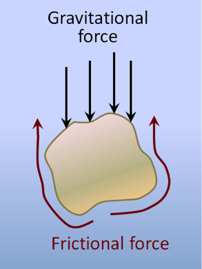](figures/14-streams-and-floods/figure-14-16.png)
Figure 14.17: How quickly a grain settles to the bottom of a stream depends on its mass (affecting the force of gravity acting on it), and the friction between the grain and the water, which slows the fall of the grain. Source: Steven Earle (2015) CC BY 4.0 view source
One of the key principles of sedimentary geology is that the ability of a moving medium (air or water) to move sedimentary particles and keep them moving is dependent on the velocity of flow. The faster the medium flows, the larger the particles it can move. As you probably know from intuition and from experience, streams that flow rapidly tend to be turbulent (flow paths are chaotic and the water surface appears rough) and the water may be muddy. In contrast, streams that flow more slowly tend to have laminar flow (straight-line flow and a smooth water surface) and clearer water. Turbulent flow is more effective than laminar flow at keeping sediments suspended within the water.
Particles within a stream are transported in different ways depending on their size (Figure 14.18). Large particles which rest on the stream bed are known as the ____bedload__. The bedload may only be transported when the flow rate is rapid and under flood conditions. They are transported by saltation (bouncing along, and colliding with other particles) and by traction__ (being pushed along by the force of the flow).
Smaller particles may rest on the bottom occasionally, where they can be transported by saltation and traction, but they can also be held in suspension in the flowing water (the ____suspended load____), especially at higher flow velocities.
Stream water also has a dissolved load, which represents (on average) about 15% of the mass of material transported, and includes ions such as calcium (Ca+2) and chloride (Cl-) in solution. The solubility of these ions is not affected by flow velocity.
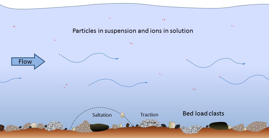](figures/14-streams-and-floods/figure-14-17.png)
Figure 14.18: Modes of transportation of sediments and dissolved ions (represented by red dots with + and – signs) in a stream . Source: Steven Earle (2015) CC BY 4.0 view source
If you look at a typical stream, there are always some sediments being deposited, some staying where they are, and some being eroded and transported. This changes over time as the discharge of the river changes in response to changing weather conditions.
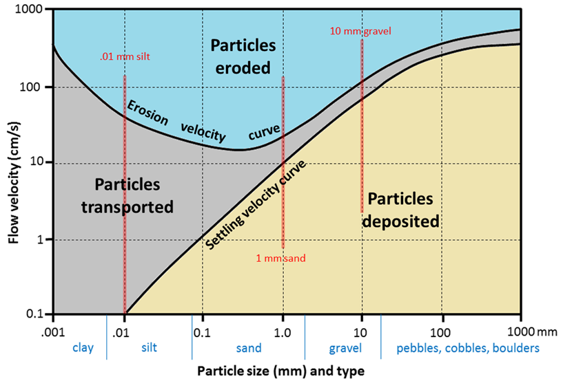
14.3.2 The Hjulström-Sundborg Diagram Summarizes What Happens to Grains of Different Sizes at Different Stream Velocities
The faster water is flowing, the larger the particles that can be kept in suspension and transported within the flowing water. However, as Swedish geographer Filip Hjulström discovered in the 1940s, the relationship between grain size and the likelihood of a grain being eroded, transported, or deposited is not as simple as one might imagine (Figure 14.19). Consider, for example, a 1 mm grain of sand. If it is resting on the bottom of the stream, it will remain there until the flow velocity is high enough to erode it (ca 20 cm/s). But once it is in suspension, that same 1 mm particle will remain in suspension as long as the velocity doesn’t drop below 10 cm/s. For a 10 mm gravel grain, the velocity is 105 cm/s to be eroded from the bed but only 80 cm/s to remain in suspension.
](figures/14-streams-and-floods/figure-14-18.png)
Figure 14.19: The Hjulström-Sundborg diagram showing the relationships between particle size and the tendency to be eroded, transported, or deposited, at different current velocities Source: Steven Earle (2015) CC BY 4.0 view source
On the other hand, a 0.01 mm silt particle only needs a velocity of 0.1 cm/s to remain in suspension, but requires 60 cm/s to be eroded. In other words, a tiny silt grain requires a greater velocity to be eroded than a grain of sand that is 100 times larger! For clay-sized particles, the discrepancy is even greater. In a stream, the most easily eroded particles are small sand grains between 0.2 mm and 0.5 mm. Anything smaller or larger requires a higher water velocity to be eroded and entrained in the flow. The reason for this is that small particles, especially tiny grains of clay, possess a net surface charge, hence experience a strong tendency to stick together, and so are difficult to erode from the stream bed.
It is important to be aware that a stream can both erode and deposit sediments at the same time. At 100 cm/s, for example, silt, sand, and medium gravel will be eroded from the stream bed and transported in suspension, coarse gravel will be transported by saltation and traction, pebbles will be both transported by saltation and traction, and will also be deposited, and cobbles and boulders will remain stationary on the stream bed.
Exercise: Understanding the Hjulström-Sundborg Diagram
Refer to the Hjulström-Sundborg diagram in Figure 14.19 to answer these questions.
- A fine sand grain (0.1 mm) is resting on the bottom of a stream bed.
- What stream velocity will it take to get this sand grain into suspension?
- Once the particle is in suspension, the velocity starts to drop. At what velocity will it finally come back to rest on the stream bed?
- A stream is flowing at 10 cm/s (which means it takes 10 s to travel 1 m).
- What size of particles can be eroded at 10 cm/s?
- What is the largest particle that, once in suspension, will remain in suspension at 10 cm/s?
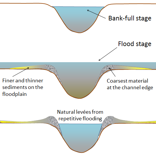
14.3.2.1 Natural Levees Form Because of Changes in Stream Velocity
A stream typically reaches its greatest velocity when it is close to flooding over its banks. This is known as the__ bank-full__ stage, as shown in Figure 14.20. When the flooding stream overtops its banks and occupies the wide area of its flood plain, the water has a much larger area to flow through and the velocity drops dramatically. As water flows from the channel out across the flood plain, it slows down and starts to deposit its sediment load. This forms an elevated bank known as a levee along the edges of the channel__. __The coarsest and thickest sediments are deposited near the channel banks, with particle size and thickness decreasing as you move further into the flood plain. People also build levees as flood control measures; the idea for this engineered solution to floods came from the naturally-build levees that form during floods.
](figures/14-streams-and-floods/figure-14-19.png)
Figure 14.20: The development of natural levees during flooding of a stream. The sediments of the levee become increasingly fine away from the stream channel, and even finer sediments — clay, silt, and very fine sand — are deposited across most of the flood plain . Source: Steven Earle (2015) CC BY 4.0 view source
14.4 Stream Types
Stream channels can be straight or curved, deep or shallow, cleared or filled with coarse sediments. The cycle of erosion has some influence on the nature of a stream, but there are several other factors that are important.
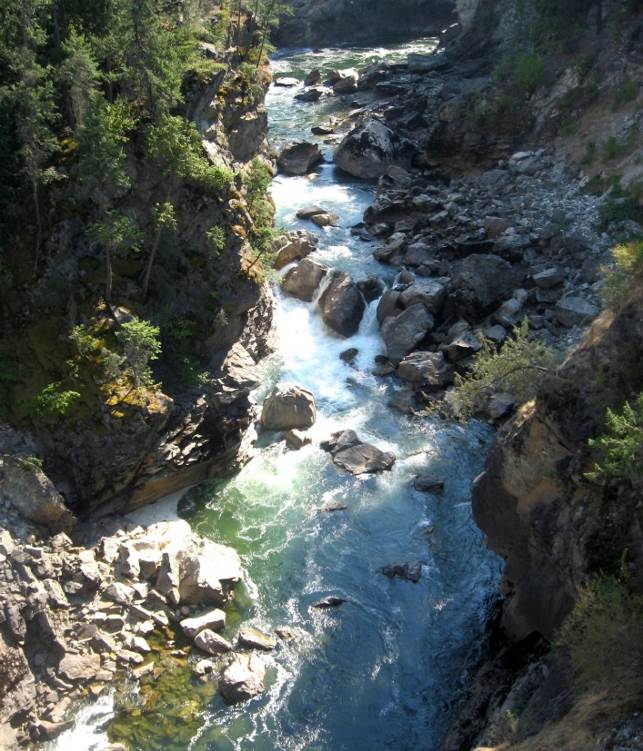
____Youthful streams__ __that are actively downcutting their channels tend to be relatively straight and are typically ungraded (meaning that rapids and waterfalls are common). As shown in Figures 14.1 and 14.21, youthful streams commonly have a step-pool morphology, meaning that the stream consists of a series of pools connected by rapids and waterfalls. They also have steep gradients, and steep and narrow V-shaped valleys. In some cases these valley walls are steep enough to be called canyons.
](figures/14-streams-and-floods/figure-14-20.jpg)
Figure 14.21: The Cascade Falls area of the Kettle River, near Christina Lake, BC. This stream has a step-pool morphology and a deep bedrock channel. Source: Steven Earle (2015) CC BY 4.0 view source
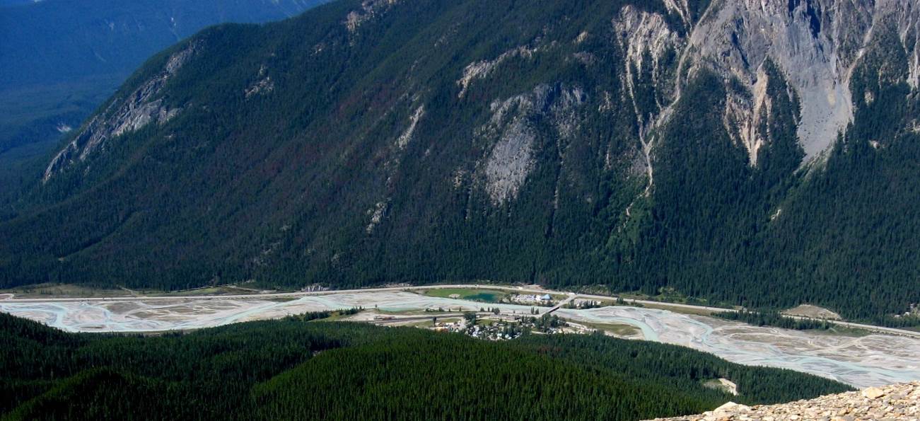
In mountainous terrain, such as that in western AB and BC, steep youthful streams typically flow into wide and relatively low-gradient U-shaped glaciated valleys. The youthful streams have high sediment loads, and when they flow into the lower-gradient glacial valleys where the velocity is no longer high enough to carry all of the sediment, ____braided____ stream patterns develop, characterized by a series of narrow channels separated by gravel bars (Figure 14.22).
](figures/14-streams-and-floods/figure-14-21.jpg)
Figure 14.22: The braided channel of the Kicking Horse River at Field, BC. Source: Steven Earle (2015) CC BY 4.0 view source
Braided streams can develop anywhere where there is more sediment than a stream is able to transport. One such environment is in volcanic regions, where explosive eruptions produce large amounts of unconsolidated material that gets washed into streams. The Coldwater River next to Mt. St. Helens in Washington State is a good example of such a braided stream (Figure 14.23).
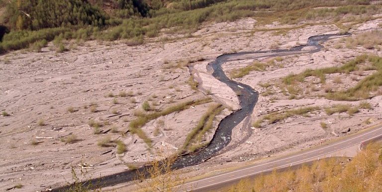](figures/14-streams-and-floods/figure-14-22.jpg)
Figure 14.23: The braided Coldwater River, Mt. St. Helens, Washington. Source: Steven Earle (2015) CC BY 4.0 view source
A stream that occupies a wide, flat flood plain with a low gradient typically carries only sand-sized and finer sediments and develops a sinuous flow pattern. As you saw in Figure 14.16, when a stream flows around a bend, the main current of the stream flows near the outside portion of the bend. This leads to erosion of the banks on the outside of the bend, and deposition of a point bar on the inside of the bend (Figure 14.24). Over time, the sinuosity of the stream becomes increasingly exaggerated, and the channel migrates throughout its flood plain, forming a meandering pattern.
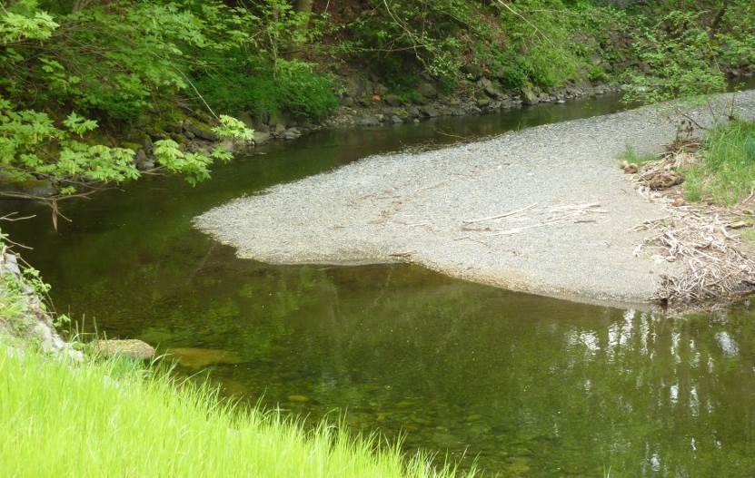](figures/14-streams-and-floods/figure-14-23.jpg)
Figure 14.24: The meandering channel of the Bonnell Creek, Nanoose, BC. The stream is flowing toward the viewer. The sand and gravel point bar must have formed when the creek was higher and the flow faster than it was when the photo was taken, as the current stream velocity is too low to carry such coarse sediments. Most erosion and deposition take place during flooding events. Source: Steven Earle (2015) CC BY 4.0 view source
A well-developed meandering river is shown in Figure 14.25. The meander in the middle of the photo has reached the point where the thin neck of land between two parts of the channel is about to be eroded through. When this happens, an oxbow lake will form. These are small cut off bends from earlier curves in the river; several are visible outside the path of the main stream in Figure 14.25.
](figures/14-streams-and-floods/figure-14-24.jpg)
Figure 14.25: The meandering channel of the Nowitna River, Alaska. Numerous oxbow lakes are present, and another meander cutoff will soon take place. Source: Oliver Kumis (2002) CC-BY-SA 2.0 view source
At the point where a stream enters a body of water such as a lake or the ocean, the flow rates drops dramatically, and sediment is deposited. Over time, as more and more sediments are deposited, the sediments form a distinctive triangular shape (with the bottom broad part of the triangle facing the ocean or lake and the point of the triangle facing upstream). This is called a delta; these are named after the Greek letter delta which is in the shape of a triangle. The Fraser River has created a large delta in BC where the river meets the Strait of Georgia (Figure 14.26). Much of the Fraser delta is very young in geological terms. Shortly after the end of the last glaciation (10,000 years ago), the delta did not extend past New Westminster. Since that time, all of the land that makes up Richmond, Delta, and parts of New Westminster and south Surrey has formed from sediment depositing from the Fraser River. You can see a more detailed description of the Fraser delta on the Geoscape Vancouver website: http://www.cgenarchive.org/vancouver-fraserdelta.html
 after NASA, September 2011 [view source ](http://bit.ly/FrasR)](figures/14-streams-and-floods/figure-14-25.jpg)
Figure 14.26: The delta of the Fraser River and the plume of sediment that extends across the Strait of Georgia. The land outlined in red has formed over the past 10,000 years. Source: Steven Earle (2015) CC BY 4.0 view source after NASA, September 2011 view source
14.4 Exercise Calculating Stream Gradients
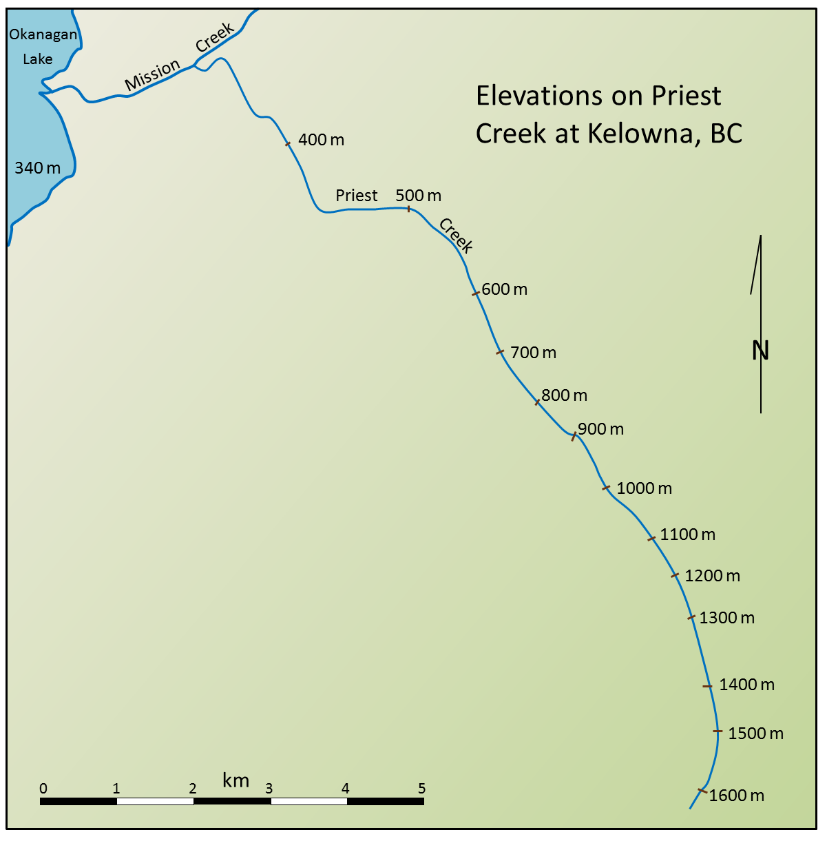 Source: Steven Earle (2015) CC BY 4.0 [view source](https://opentextbc.ca/geology/wp-content/uploads/sites/110/2015/08/Stream-Gradients.png)](https://openpress.usask.ca/app/uploads/sites/29/2017/05/Stream-Gradients.png)
Figure 14.27: Source: Steven Earle (2015) CC BY 4.0 view source
The gradient is the key factor controlling stream velocity, and stream velocity controls sediment erosion and deposition. This map shows the elevations of Priest Creek in the Kelowna area. The length of the creek between 1,600 m and 1,300 m elevation is 2.4 km, so the gradient is (1,600 m - 1,300 m)/2.4 km = 125 m/km.
- Use the scale bar to estimate the distance between 1,300 m and 600 m and calculate the gradient between these two elevations.
- Estimate the gradient between 600 and 400 m.
- Estimate the gradient between 400 m on Priest Creek and the point where Mission Creek enters Okanagan Lake.
14.5 Flooding
The discharge levels of streams are highly variable depending on the time of year and on variations in the weather from one year to the next. In Canada, most streams show discharge variability similar to that of the Stikine River in northwestern BC, illustrated in Figure 14.28. The Stikine River has its lowest discharge levels in the depths of winter when freezing conditions persist throughout most of its drainage basin. Discharge starts to rise slowly in May, and then rises dramatically through the late spring and early summer as the winter snow melts. For the year shown, the minimum discharge of the Stikine River was 56 m3/s in March, and the maximum was 37 times higher at 2,470 m3/s in May.
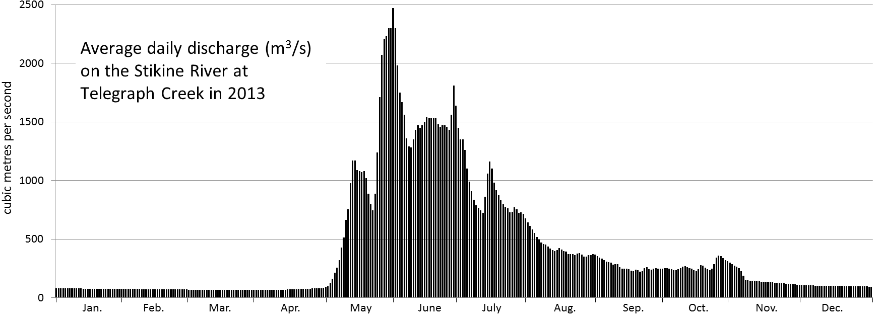 from data at Water Survey of Canada, Environment Canada [view source](http://www.ec.gc.ca/rhc-wsc/)](figures/14-streams-and-floods/figure-14-26.png)
Figure 14.28: Variations in discharge of the Stikine River during 2013. Source: Steven Earle (2015) CC BY 4.0 view source from data at Water Survey of Canada, Environment Canada view source
Streams in coastal areas of southern British Columbia show a very different pattern from those in most of the rest of the country. In this region, the drainage basins receive a lot of rain (rather than snow) during the winter and also do not remain entirely frozen throughout the winter. The Qualicum River on Vancouver Island typically has its highest discharge levels in January or February and its lowest levels in late summer (Figure 14.29). In 2013, the minimum discharge of the Qualicum River was 1.6 m3/s in August, and the maximum was 34 times higher at 53 m3/s in March.
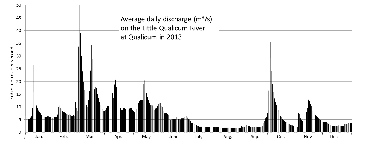, from data at Water Survey of Canada, Environment Canada [view source](http://www.ec.gc.ca/rhc-wsc/)](figures/14-streams-and-floods/figure-14-27.png)
Figure 14.29: Variations in discharge of the Qualicum River during 2013. Source: Steven Earle (2015) CC BY 4.0 view source, from data at Water Survey of Canada, Environment Canada view source
When a stream’s discharge increases, both the water level (____stage_) and the velocity increase as well. Rapidly flowing streams become muddy, and large volumes of sediment are transported both in suspension and along the stream bed. In extreme situations, the water level reaches the top of the stream’s banks (the _bank-full stage____, see Figure 14.20), and if it rises further, it will overflow the banks and floods the surrounding terrain. In the case of mature or old-age streams, this could include a vast area of relatively flat ground known as a flood plain, which is the area that is typically covered with water during a major flood. Since fine river sediments are deposited on flood plains, they are ideally suited for agriculture, and thus are typically occupied by farms and residences, and in many cases, by towns or cities. Such infrastructure is highly vulnerable to damage from flooding, and the people that live and work there are at risk.
Most streams in Canada have the greatest risk of flooding in the late spring and early summer when stream discharges rise in response to melting snow. In some cases, this is exacerbated by spring storms. In years when melting is especially fast and/or spring storms are particularly intense, flooding can be very severe.
One of the worst floods in Canadian history took place in the Fraser Valley of BC in late May and early June of 1948. The early spring of that year had been cold, and a large snow pack in the interior was slow to melt. In mid-May, temperatures rose quickly and melting was accelerated by rainfall. Fraser River discharge levels rose rapidly over several days during late May, and the dykes built to protect the valley were breached in a dozen places. Approximately one-third of the flood plain was inundated, and many homes and other buildings were destroyed, but there were no deaths.
The Fraser River flood of 1948, which was the worst flood in the Fraser Valley in the past century, was followed by very high river levels in 1950 and 1972, and by relatively high levels several times since then, the most recent being 2007 (Table 14.1). In the years following 1948, millions of dollars were spent repairing and raising the existing dykes and building new ones. Since then damage from flooding in the Fraser Valley has been relatively limited.
| Rank | Year | Month | Day | Stage (m) | Discharge (m3/s) |
|---|---|---|---|---|---|
| 1 | 1948 | May | 31 | 11.0 | 15200 |
| 2 | 1972 | Jun | 16 | 10.1 | 12900 |
| 3 | 1950 | Jun | 20 | 9.9 | 12500 |
| 4 | 1964 | Jun | 21 | 9.6 | 11600 |
| 5 | 1997 | Jun | 5 | 9.5 | 11300 |
| 6 | 1955 | Jun | 29 | 9.4 | 11300 |
| 7 | 1999 | Jun | 22 | 9.4 | 11000 |
| 8 | 2007 | Jun | 10 | 9.3 | 10850 |
| 9 | 1974 | Jun | 22 | 9.3 | 10800 |
| 10 | 2002 | Jun | 21 | 9.2 | 10600 |
Serious flooding occurred in July 1996 in the Saguenay-Lac St. Jean region of Quebec. In this case, the floods were caused by two weeks of heavy rainfall followed by one day of exceptional rainfall. On July 19, 1996 there was 270 mm of rain, equivalent to the region’s normal rainfall for the entire month of July. Ten deaths were attributed to the Saguenay floods, and the economic toll was estimated at $1.5 billion.
Just a year after the Saguenay floods, the Red River in Minnesota, North Dakota, and Manitoba reached its highest level since 1826. As is typical for the Red River, the 1997 flooding was due to rapid snowmelt. Due to the south to north flow of the river, the flooding starts in Minnesota and North Dakota, where melting begins earlier, then extends northwards. The residents of Manitoba had plenty of warning that the 1997 flood was coming because there was severe flooding at several locations on the U.S. side of the border.
After the 1950 Red River flood, the Manitoba government built a channel around the city of Winnipeg to reduce the potential of flooding in the city (Figure 14.30). Known as the Red River Floodway, the channel was completed in 1964 at a cost of $63 million. Since then it has been used many times to alleviate flooding in Winnipeg, and is estimated to have saved many billions of dollars in flood damage. The massive 1997 flood (Figure 14.30, right side) was almost too much for the floodway; in fact the amount of water diverted was greater than the designed capacity. The floodway has recently been expanded so that it can be used to divert even more of the Red River’s flow away from Winnipeg.
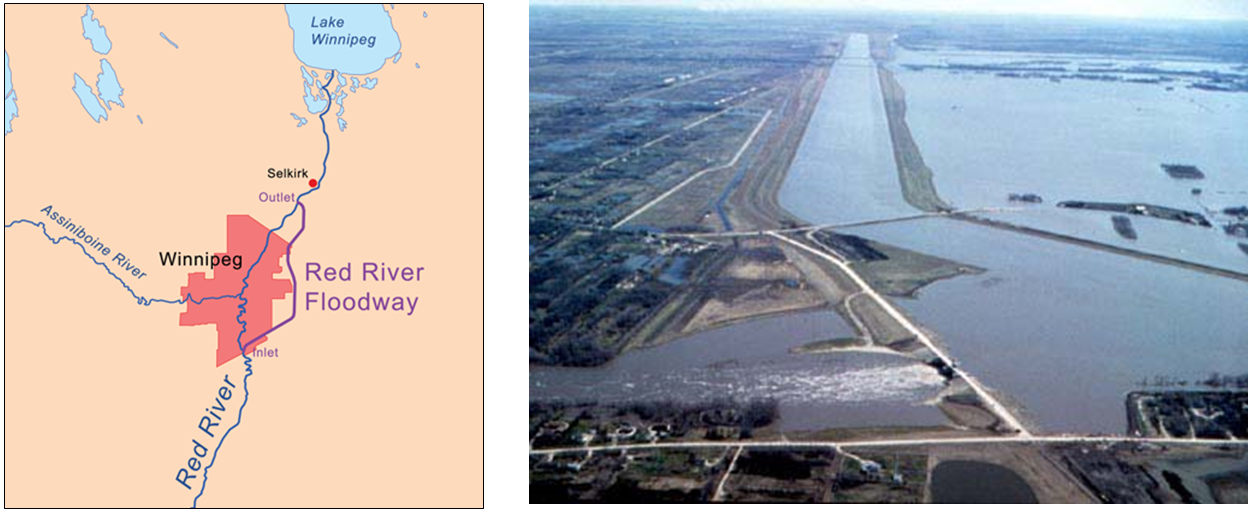 (right) Natural Resources Canada 2012, courtesy of the Geological Survey of Canada (Photo 2000-118 by G.R. Brooks ).](figures/14-streams-and-floods/figure-14-28.png)
Figure 14.30: (left) map of the Red River Floodway around Winnipeg, Manitoba; (right) aerial view of the southern (inlet) end of the floodway during the 1997 Red River flood. Sources: (left) Wikimedia user “Kmusser” (2007) CC BY 2.5view source, (right) Natural Resources Canada 2012, courtesy of the Geological Survey of Canada (Photo 2000-118 by G.R. Brooks ).
Canada’s most costly flood ever was the June 2013 flood in southern Alberta. The flooding was initiated by snowmelt and worsened by heavy rains in the Rockies due to an anomalous flow of moist air from the Pacific and the Caribbean. At Canmore, AB rainfall amounts exceeded 200 mm in 36 hours, and at High River, AB 325 mm of rain fell in 48 hours.
](figures/14-streams-and-floods/figure-14-29.png)
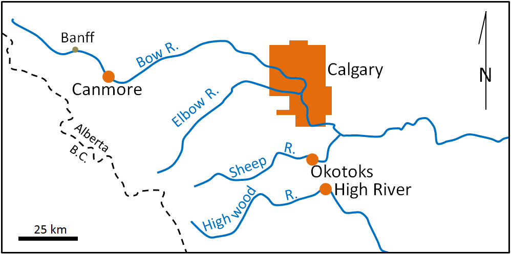
Figure 14.31: Map of the communities most affected by the 2013 Alberta floods (in orange) Source: Steven Earle (2015) CC BY 4.0 view source
In late June and early July, the discharges of several rivers in the area, including the Bow River in Banff, Canmore, and Exshaw, the Bow and Elbow Rivers in Calgary, the Sheep River in Okotoks, and the Highwood River in High River, reached levels that were 5 to 10 times higher than normal for that time of year (see Exercise 14.5). Large areas of Calgary, Okotoks, and High River were flooded, and five people died (see Figures 14.31 and 14.32). The cost of the 2013 flood is estimated to be approximately $5 billion.
 (right) Wikimedia user "Stephanie N. Jones" (2013) CC BY-SA 3.0 [view source ](https://en.wikipedia.org/wiki/2013_Alberta_floods#/media/File:Okotoks_-_June_20,_2013_-_Flood_waters_in_local_campground_playground-03.JPG)](figures/14-streams-and-floods/figure-14-30.png)
Figure 14.32: Flooding in Calgary (June 21, left) and Okotoks (June 20, right) during the 2013 southern Alberta flood. Sources: (left) Wikimedia user Ryan L.C. Quan (2013) CC BY-SA 3.0 view source (right) Wikimedia user “Stephanie N. Jones” (2013) CC BY-SA 3.0 view source
Flood Mitigation
One of the things that the 2013 flood of the Bow River teaches us is that we cannot predict when a flood will occur nor how big it will be, so in order to minimize damage and casualties we need to be prepared. Some ways of preparing include:
- Mapping flood plains and not building within them
- Building dykes or dams where necessary
- Monitoring the winter snowpack, the weather, and stream discharges
- Creating emergency plans
- Educating the public on how to prepare for and respond to the threat of flooding
Exercise: Flood Probability on the Bow River
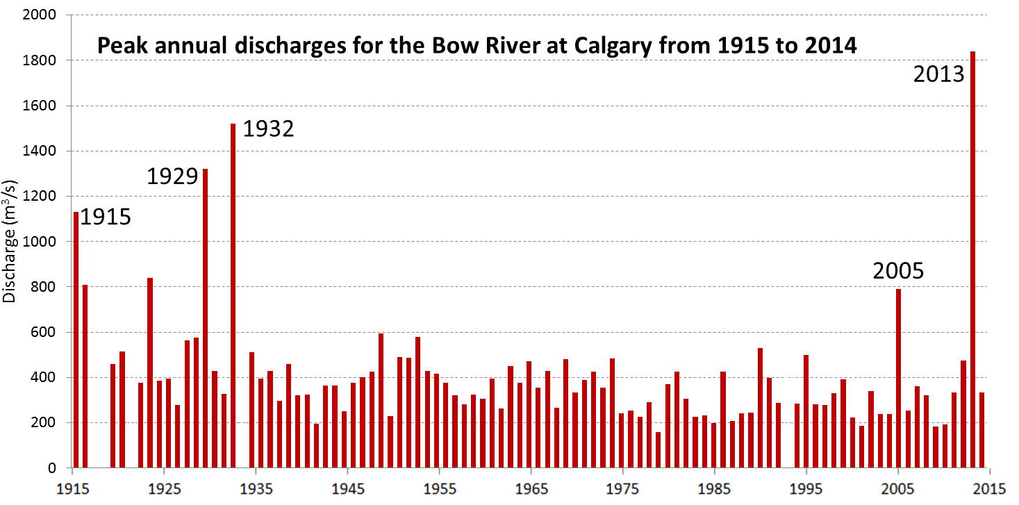
The graph below shows the highest discharge per year between 1915 and 2014 of the Bow River in Calgary. Using this data set, we can calculate the recurrence interval (Ri) for any particular flood magnitude using the equation: Ri = (n+1)/r (where n is the number of floods in the record being considered, and r is the rank of the particular flood). There are a few years missing in this record, so the actual number of floods is 95.
The largest flood recorded along the Bow River over that period of time was the one in 2013, reaching a peak flow rate of 1,840 m3/s on June 21. Ri for this flood is (95+1)/1 = 96 years. The probability of such a flood in any future year is 1/Ri x 100%, which is 1%. The fifth largest flood was just a few years earlier in 2005, at 791 m3/s. Ri for this flood is (95+1)/5 = 19.2 years. The recurrence probability of a flood of this magnitude is thus 5%.
- Calculate the recurrence interval for the second largest flood (1932, 1,520 m3/s).
- What is the probability that a flood of 1,520 m3/s will happen next year?
- Examine the 100-year trend for floods along the Bow River. If you ignore the major floods (the labelled ones), what is the general trend of peak discharges over this time?
 Source: Steven Earle (2015) CC BY 4.0[ view source](http://wateroffice.ec.gc.ca/search/searchDownload_e.html), from data at Water Surveys of Canada, Environment Canada [view source ](http://wateroffice.ec.gc.ca/search/searchDownload_e.html)](https://openpress.usask.ca/app/uploads/sites/29/2017/05/Water-Surveys-of-Canada.png)
Figure 14.33: Source: Steven Earle (2015) CC BY 4.0view source, from data at Water Surveys of Canada, Environment Canada view source
14.6 Summary
The topics covered in this chapter can be summarized as follows:
14.6.1 The Hydrological Cycle
Water is stored in the oceans, glacial ice, the ground, lakes, rivers, and the atmosphere. Its movement is powered by solar energy and gravity.
14.6.2 Drainage Basins
All of the precipitation that falls within a drainage basin flows into the stream that drains that area. Stream drainage patterns are determined by the type of rock within the basin. Over geological time, streams change the landscape that they flow within, and eventually they become graded, meaning their profile becomes a smooth curve. A stream can lose that gradation if there is renewed uplift or if their base level changes for some other reason such as construction of a dam downstream.
14.6.3 Stream Erosion and Deposition
The processes of erosion and deposition of particles within streams are primarily driven by the velocity of the stream water. Erosion and deposition of different-sized particles can happen simultaneously in a stream. Some particles are moved along the bottom of a river while others are carried in suspension. It takes a greater velocity of water to erode a particle from a stream bed than it does to keep it in suspension. Ions are also transported in solution. When a stream rises and then occupies its flood plain, the velocity of water over the flood plains slows and natural levees form along the edges of the stream channel.
14.6.4 Stream Types
Youthful streams in steep areas erode most rapidly downwards, and they tend to have steep, rocky, and relatively straight channels. Where sediment-rich streams empty into areas with lower gradients, braided streams can form. Meandering streams are common in areas with even lower gradients where silt and sand are the dominant sediments. Meandering streams erode the walls of their channels more rapidly than the channel base. Deltas form where streams flow into standing water.
14.6.5 Flooding
Most streams in Canada have their highest discharge rates in spring and early summer, although the highest discharge in many of BC’s coastal streams is in the winter. Floods happen when a stream rises high enough to spill over its banks and spread across its flood plain. Some of the more significant floods in Canada include the Fraser River flood of 1948, the Saguenay River flood of 1996, the Red River flood of 1997, and the Alberta floods of 2013. We can estimate the probability of a specific flood level based on the record of past floods, and we can take steps to minimize the impacts of flooding such as building floodways to divert excess water and not building in flood-prone areas.
14.7 Chapter Review Questions
What is the proportion of liquid fresh water on Earth expressed as a percentage of all water on Earth?
What percentage of this fresh water is groundwater?
What type of rock, and what processes, can lead to the formation of a trellis drainage pattern?
Why do many of the streams in the southwestern part of Vancouver Island empty into the ocean over waterfalls?
Where would you expect to find the fastest water flow along a straight stretch of a stream?
Sand grains can be moved by traction and saltation. What minimum stream velocity is required to move 1 mm sand grains?
If the flow velocity of a stream is 1 cm/s, what sizes of particles can be eroded, what sizes can be transported if they are already in suspension, and what sizes of particles cannot be moved at all?
Under what circumstances might a braided stream develop?
How would the gradient of a stream be affected if a meander is bypassed?
The elevation of the Fraser River at Hope is 41 m. From there it flows approximately 147 km to the sea. What is the average gradient of the river (m/km) over this distance?
How do BC’s coastal streams differ from most of the rest of the streams in Canada in terms of their annual flow patterns? Why?
Why do most serious floods in Canada happen in late May, June, or early July?
There is a 65-year record of peak annual discharges along the Ashnola River near Princeton, BC. During this time, the second highest discharge recorded was 175 m3/s. Based on this information, what is the recurrence interval (Ri) for this discharge level, and what is the probability that there will be a similar peak discharge next year?
14.8 Answers to Chapter Review Questions
Approximately 1% of the Earth’s water is liquid fresh water.
Approxmately 30% of the Earth’s fresh water is groundwater.
A trellis drainage pattern typically forms on sedimentary rock that has been tilted and eroded.
Many of the streams in the southwestern part of Vancouver Island flow to the ocean as waterfalls because the land has been uplifted relative to sea level over the past several thousand years.
The fastest water flow on a straight stretch of a stream will be in the middle of the stream near the surface.
1 mm sand grains will be eroded if the velocity if over 20 cm/s and will be kept in suspension as long as the velocity is over 10 cm/s.
If the flow velocity is 1 cm/s particles less than 0.1 mm (fine sand or finer) can be transported, while those larger than 0.1 mm cannot. At this velocity no particles can be eroded.
A braided stream can develop where there is more sediment available than can be carried in the amount of water present at the rate at which that water is flowing. This may happen where the gradient drops suddenly, or where there is a dramatic increase in the amount of sediment available (e.g., following an explosive volcanic eruption).
If a meander is cut off it reduces the length of a stream so it increases the gradient.
The average gradient of the Fraser River between Hope and the Pacific Ocean is 0.28 m/km (or 28 cm/km).
In coastal regions of B.C. the highest levels of precipitation are in the winter, and large parts of most drainage basins are not frozen solid. As a result stream discharges tend to be greatest in the winter.
In most parts of Canada winter precipitation is locked up in snow until the melt season begins, and depending on the year and the location that happens in late spring or early summer. If the thaw is delayed because of a cold spring, and then happens very quickly, flooding is likely. Some regions also receive heavy rainfall during this period of the year.
Ri = (n+1)/r (where n is the length of the record) and r is the rank of the flood in question. In the Ashnola River case Ri = (65+1)/2 = 33. The probability of such a flood next year is 1/Ri, or 1/33 which is 0.03 or 3%.