Chapter 4 Plate Tectonics
Adapted from Physical Geology, First University of Saskatchewan Edition (Karla Panchuk) and Physical Geology (Steven Earle)
. Click the image for more attributions._](figures/04-plate-tectonics/figure-4-1.png)
Figure 4.1: Iceland is known for its volcanoes, which are present because Iceland is located on the Mid-Atlantic Ridge, where the Atlantic Ocean is spreading apart and new crust is forming. In fact, Iceland exists because that volcanic activity has built up the island from the ocean floor. Iceland is cut by rift zones (white lines on the map at left) where the island is splitting apart along with the rest of the Atlantic Ocean. Rift zones are marked by belts of young volcanic rocks (dark green). You can stand on a rift zone if you visit Thingvellir National Park (right). Rifting has produced a valley where the crust has settled downward. The margins of the North American and Eurasian tectonic plates are visible as ridges on either side of the valley. The photographer was standing on a ridge on the North American side. Source: Karla Panchuk (2018) CC BY-SA 4.0. Photo: Ruth Hartnup (2005) CC BY 2.0 view source. Click the image for more attributions.
Learning Objectives
After reading this chapter and answering the review questions at the end, you should be able to:
- Discuss the early evidence for continental drift, and Alfred Wegener’s role in promoting this theory.
- Describe other models that were used early in the 20th century to understand global geological features.
- Summarize the geological advances that provided the basis for understanding the mechanisms of plate tectonics, and the evidence that plates and are constantly being created and destroyed.
- Describe the seven major plates, including their size, motion, and the types of boundaries between them.
- Describe the geological processes that take place at divergent and convergent plate boundaries, and explain why transform faults exist
- Explain how supercontinents form and how they break apart.
- Explain why tectonic plates move.
Plate tectonics is the model or theory that we use to understand how our planet works: it explains the origins of continents and oceans, the origins of folded rocks and mountain ranges, the presence of different kinds of rocks, the causes and locations of earthquakes and volcanoes, and changes in the positions of continents over time. So… everything!
The theory of plate tectonics was proposed to the geological community more than 100 years ago, so it may come as a surprise that an idea underpinning the study of Earth today did not become an accepted part of geology until the 1960s. It took many decades for this theory to become accepted for two main reasons. First, it was a radically different perspective on how Earth worked, and geologists were reluctant to entertain an idea that seemed preposterous in the context of the science of the day. The evidence and understanding of Earth that would have supported plate tectonic theory simply didn’t exist until the mid-twentieth century. Second, their opinion was affected by their view of the main proponent, Alfred Wegener. Wegener was not trained as a geologist, so he lacked credibility in the eyes of the geological community. Alfred Wegener was also German, whereas the geological establishment was centred in Britain and the United States- and Britain and the United States were at war with Germany in the first part of the 20th century. In summary, plate tectonics was an idea too far ahead of its time, and delivered by the wrong messenger.
4.1 Alfred Wegener’s Arguments for Plate Tectonics
Alfred Wegener (1880-1930; Figure 4.2) earned a PhD in astronomy at the University of Berlin in 1904, but had a keen interest in geophysics and meteorology, and focused on meteorology for much of his academic career.
_](figures/04-plate-tectonics/figure-4-2.jpg)
Figure 4.2: Alfred Wegener during a 1912-1913 expedition to Greenland. Source: Alfred Wegener Institute (2008) Public Domain view source
In 1911 Wegener happened upon a scientific publication that described matching Permian-aged terrestrial fossils in various parts of South America, Africa, India, Antarctica, and Australia. He concluded that because these organisms could not have crossed the oceans to get from one continent to the next, the continents must have been joined in the past, permitting the animals to move from one to the other (Figure 4.3). Wegener envisioned a supercontinent made up of all the present day continents, and named it Pangea (meaning “all land”). He described the motion of the continents reconfiguring themselves as continental drift.
_](figures/04-plate-tectonics/figure-4-3.gif)
Figure 4.3: The distribution of several Permian terrestrial fossils that are present in various parts of continents now separated by oceans. During the Permian, the supercontinent Pangea included the supercontinent Gondwana, shown here, along with North America and Eurasia. Source: J.M. Watson, USGS (1999) Public Domainview source
Wegener pursued his idea with determination, combing libraries, consulting with colleagues, and making observations in an effort to find evidence in support of it. He relied heavily on matching geological patterns across oceans, such as sedimentary strata in South America matching those in Africa, North American coalfields matching those in Europe, the mountains of Atlantic Canada matching those of northern Britain—both in structure and rock type—and comparisons of rocks in the Canadian Arctic with those of Greenland (Figure 4.4).
 comparing rock types on Canadian Arctic Islands and Greenland. _Source: Karla Panchuk (2018) CC BY 4.0. Click the image for more attributions._](figures/04-plate-tectonics/figure-4-4.png)
Figure 4.4: Diagram from Alfred Wegener’s book Die Entstehung der Kontinente und Ozeane comparing rock types on Canadian Arctic Islands and Greenland. Source: Karla Panchuk (2018) CC BY 4.0. Click the image for more attributions.
Wegener also called upon evidence for the Carboniferous and Permian (~300 Ma) Karoo Glaciation from South America, Africa, India, Antarctica, and Australia (Figure 4.5). He argued that this could only have happened if these continents were once all connected as a single supercontinent. He also cited evidence (based on his own astronomical observations) that showed that the continents were moving with respect to each other, and determined a separation rate between Greenland and Scandinavia of 11 m per year, although he admitted that the measurements were not accurate. (The separation rate is actually about 2.5 cm per year.)
. Click the image for terms of use._](figures/04-plate-tectonics/figure-4-5.png)
Figure 4.5: Carboniferous and Permian Karoo Glaciation in the southern hemisphere. Paleogeographic reconstruction for 306 million years ago._ Source: Cropped from C. R. Scotese, PALEOMAP Project (www.scotese.com) view source. Click the image for terms of use._
Wegener first published his ideas in 1912 in a short book called Die Entstehung der Kontinente (The Origin of Continents), and then in 1915 in Die Entstehung der Kontinente und Ozeane (The Origin of Continents and Oceans). He revised this book several times up to 1929. It was translated into French, English, Spanish, and Russian in 1924.
The main criticism of Wegener’s idea was that he could not explain how continents could move. Remember that, as far as anyone was concerned, Earth’s crust was continuous, not broken into plates. Thus, any mechanism Wegener could think of would have to fit with that model of Earth’s structure. Geologists at the time were aware that continents were made of different rocks than the ocean crust, and that the material making up the continents was less dense, so Wegener proposed that the continents were like icebergs floating on the heavier ocean crust. He suggested that the continents were moved by the effect of Earth’s rotation pushing objects toward the equator, and by the lunar and solar tidal forces, which tend to push objects toward the west. However, it was quickly shown that these forces were far too weak to move continents, and without any reasonable mechanism to make it work, Wegener’s theory was quickly dismissed by most geologists of the day.
Alfred Wegener died in Greenland in 1930 while carrying out studies related to glaciation and climate. At the time of his death, his ideas were tentatively accepted by a small minority of geologists, and firmly rejected by most. But within a few decades that was all to change.
4.2 Global Geological Models of the Early 20th Century
The untimely death of Alfred Wegener did not solve any problems for those who opposed his ideas, because they still had some inconvenient geological truths to deal with. One of those was explaining the distribution of terrestrial species across five continents that are currently separated by hundreds or thousands of kilometres of ocean water, and another was explaining the origin of extensive fold-belt mountains, such as the Appalachians, the Alps, the Himalayas, and the Canadian Rockies.
Before we continue, it is important to know what was generally believed about global geology before plate tectonics. At the beginning of the 20th century, geologists had a good understanding of how most rocks were formed and understood their relative ages through interpretation of fossils, but there was considerable controversy regarding the origin of mountain chains, especially fold-belt mountains. At the end of the 19th century, one of the prevailing views on the origin of mountains was the theory of contractionism — the idea that since Earth is slowly cooling, it must also be shrinking. In this scenario, mountain ranges had formed like the wrinkles on a dried-up apple. Oceans formed above parts of former continents that had settled downward and become submerged.
While this hypothesis helped to address the dilemma of the terrestrial fossils by explaining how continents once connected could now be separated by oceans, it came with its own set of problems. One problem was that Earth wasn’t cooling fast enough to create the necessary amount of shrinking. Another problem was the principle of isostasy (already understood for several decades; see Section 3.5 for a review of isostasy), which wouldn’t allow blocks of continental crust to sink in the way necessary for oceans to form in accordance with contractionist theory.
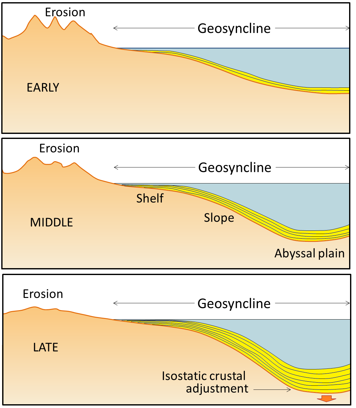
Another widely held view was permanentism, the idea that the continents and oceans have always been generally the same as they are today. This view incorporated a mechanism for creation of mountain chains known as the geosyncline theory. A geosyncline is a thick (potentially 1000s of metres) deposit of sediments and sedimentary rocks, typically situated along the edge of a continent, and derived from continental weathering (Figure 4.6).
_](figures/04-plate-tectonics/figure-4-6.png)
Figure 4.6: The development of a geosyncline along a continental margin. (Note that a geosyncline is not related to a syncline, which is a downward fold in rocks.) Source: Steven Earle (2015) CC BY 4.0 view source
The idea that geosynclines developed into fold-belt mountains originated in the middle of the 19th century. It was first proposed by James Hall and later elaborated upon by Dwight Dana, both of whom worked extensively in the Appalachian Mountains of the eastern United States. The process of converting a geosyncline into a mountain belt was believed to involve compression by forces pushing from either side, causing sedimentary layers within the geosyncline to fold up. In 1937, Philip Kuenen published a paper of experiments with layers of paraffin wax to test how this might work. He was able to cause layers within a geosyncline to fold up as the geosyncline deepened and became more tightly folded during the experiment (Figure 4.7).
._](figures/04-plate-tectonics/figure-4-7.png)
Figure 4.7: Simulation of mountain building within a geosyncline using layers of wax. Left- A sequence of photographs showing deformation in the wax layers as pistons apply increasing amounts of compression from the side. Right- Close-up view of slices through the wax layers at the end of the experiment, showing that stiffer white layers of wax folded in a way that resembled the folds in mountain belts. Source: Karla Panchuk (2018) CC BY 4.0. Photographs from Kuenen (1937) Public Domain view source.
The problem with the geosynclinal hypothesis for mountain building is that the lateral forces required to cause the compression were never adequately explained. Kuenen compressed the wax layers in his experiment by using pistons that pushed horizontally from either side, but described that mechanism as unrealistic. He explained that the pistons were just to get the process started within the experiment, and that in nature the main force was likely that of gravity pulling the geosyncline downward, drawing the sides together as it folded. When the sides were drawn together, this provided the compression to fold the sediments within the geosyncline. He couldn’t specify how the process got started in nature, but suggested that there could be a variety of reasons for an irregularity in the crust to respond to forces in such a way that would trigger downward sagging and folding.
Proponents of the geosyncline theory of mountain formation—and there were many well into the 1960s—also had the problem of explaining the intercontinental terrestrial fossil matchups. The explanation offered was that land bridges had once linked the continents, permitting animals and plants to migrate back and forth. One proponent of this idea was the American naturalist Ernest Ingersoll. Referring to evidence of past climate changes, Ingersoll contributed the following to the 1918-20 edition of the Encyclopedia Americana:
The most interesting feature of these changes, however, is that by which, now and again, the Old World was connected with the New by necks or spaces of land, known as “land-bridges”; especially as these permitted an interchange of plants and animals, giving to us many new ones from the other side of the ocean, including, finally, man himself.
A problem with the land-bridge hypothesis is that there is no evidence of land bridges that could account for the fossil distribution patterns. The world’s oceans are approximately 4 km deep on average, so the underwater slopes leading up to a land bridge would have to have been at least 10s of km wide in most places, and many times that in others. Even if flooded, a land bridge of that size would still be visible in the shape of ocean-floor terrain. Isostasy would not permit such a land bridge to sink down without leaving a trace.
We do know the locations of some past land bridges, but they were very different from the ones that would be required for this hypothesis. They are bridges such as the flooded Bering Strait land bridge, which is beneath only 30 to 50 m of water, and was exposed when sea levels were much lower because of water being locked in polar ice caps during the last major glaciation event. The narrowest point of the Bering Strait is 82 km wide. The shortest distance between South America and Africa is more than 2800 km.
_](figures/04-plate-tectonics/figure-4-8.png)
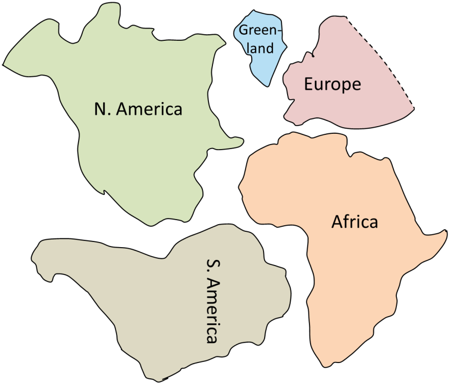
(\#fig:figure-4-8)Mesozoic continent shapes. _Source: Steven Earle (2015) CC BY 4.0 [view source](http://opentextbc.ca/geology/wp-content/uploads/sites/110/2015/07/image0111.png)_
4.3 Geological Renaissance of the Mid-20th Century
Two key areas of research ultimately led to the acceptance of continental drift, and the formulation of plate tectonic theory. One was the study of paleomagnetism, the record of Earth’s magnetic field through time. The other was exploration of the ocean floor.
4.3.1 Paleomagnetism (Remnant Magnetism)
](figures/04-plate-tectonics/figure-4-9.png)
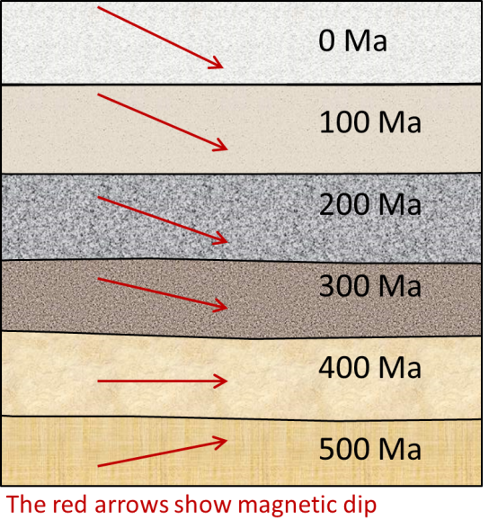
Figure 4.8: Rock layers recording remnant magnetism. The red arrows represent the direction of the vertical component of Earth’s magnetic field. The oldest rock has a magnetic dip characteristic of the southern hemisphere, but over time the dip changes, indicating that the rocks moved toward magnetic north. Source: Steven Earle (2015) CC BY 4.0 view source
When rocks form, some of the minerals that make them up can become aligned with the Earth’s magnetic field, just like a compass needle pointing to north. This happens to the mineral magnetite (Fe3O4) when it crystallizes from magma. Once the rock cools the crystals are locked in place. This means that if the rock moves, the crystals can’t realign themselves, and they retain a remnant magnetism. This would be like jamming your compass needle so that if you turned away from north, the needle would turn with you rather than continuing to point north.
Rocks like basalt, which cool from a high temperature and commonly have relatively high levels of magnetite, are particularly susceptible to being magnetized in this way. However, even sediments and sedimentary rocks can take on remnant magnetism as long as they have small amounts of magnetic minerals, because the magnetic grains can gradually become lined up with Earth’s magnetic field as the sediments are deposited.
By studying both the horizontal and vertical components of the remnant magnetism, one can tell not only the direction to magnetic north at the time of the rock’s formation, but also the latitude where the rock formed relative to magnetic north. Remember that the vertical component of the magnetic field points more sharply downward the closer it is to the magnetic north pole. Figure 4.8 shows the vertical component of remnant magnetism in a sequence of rocks. Notice that the arrow starts out at 500 Ma pointing slightly upward. This means that the rocks were in the southern hemisphere. As the rocks get younger, the arrow tilts toward horizontal, and then points downward. This indicates that the rocks were getting progressively closer to the north magnetic pole.
4.3.1.1 Apparent Polar Wandering Paths
In the early 1950s, a group of geologists from Cambridge University, including Keith Runcorn, Ted Irving,3 and several others, started looking at the remnant magnetism of Phanerozoic British and European volcanic rocks, and collecting paleomagnetic data. Using an analysis similar to that in Figure 4.8, they noticed that rocks of different ages sampled from the same general area showed very different magnetic pole positions (the green line in Figure 4.9). They assumed this meant that Earth’s magnetic pole had moved around significantly over time along polar wandering paths, rather than staying close to the geographic north pole as it does today. At the time, geophysical models suggested that the magnetic poles did not need to be aligned with the rotational poles, so this wasn’t an unreasonable conclusion, given what was known.
](figures/04-plate-tectonics/figure-4-10.png)
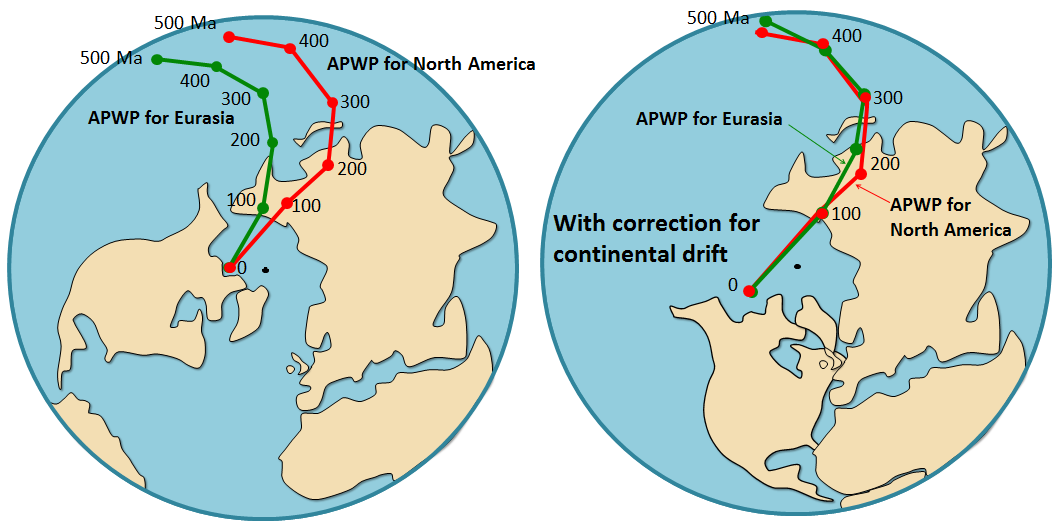
Figure 4.9: Apparent polar-wandering paths (APWP) for Eurasia and North America. The view is from the geographic north pole (black dot) looking down. Dots along each path show the location of magnetic north as determined from paleomagnetic data. Left- Data from Eurasia and North America agree on the location of magnetic north today (time 0), but not at any time in the past. Right- Once continent motion has been accounted for, there is agreement in data from Eurasia and North America on the location of magnetic north over the past 500 million years. Source: Steven Earle (2015) CC BY 4.0 view source
Runcorn and colleagues extended their paleomagnetic studies to North America, and began to realize that their initial conclusion had a problem. Notice that on the right of Figure 4.9 the polar wandering path for North America (in red) does not match the path for Eurasia (in green). For example, data from North America suggest that 200 Ma ago, magnetic north was somewhere in China, whereas data from Europe said it was in the Pacific Ocean. There could only have been one magnetic north pole position at 200 Ma, therefore the only way to explain the discrepancy was if Europe and North America moved along different paths during this time while the pole stayed in more or less the same location.
The polar wandering paths were not actually records of the pole moving, they just looked that way, so the paths are now referred to as apparent polar wandering paths (APWP). Subsequent paleomagnetic work showed that unique apparent polar wandering paths can be derived from rocks in South America, Africa, India, and Australia. In 1956, Runcorn became a proponent of continental drift. There was simply no other way to explain the data.
This paleomagnetic work of the 1950s was the first new evidence in favour of continental drift, and it led a number of geologists to start thinking that the idea might have some merit. Nevertheless, for a majority of geologists, this type of evidence was not sufficiently convincing to get them to change their views.
4.3.2 Ocean Basin Geology and Geography
During the 20th century, our knowledge and understanding of the ocean basins and their geology increased dramatically. Before 1900 we knew virtually nothing about the bathymetry (the hills and valleys of the ocean floor) and geology of the oceans. By the end of the 1960s, we had detailed maps of the topography of the ocean floors, a clear picture of the geology of ocean floor sediments and the solid rocks beneath them, and almost as much information about the geophysical nature of ocean rocks as of continental rocks.
4.3.2.1 Acoustic Depth Sounding
Up until the 1920s, ocean depths were measured using weighted lines dropped overboard. In deep water this is a painfully slow process and the number of soundings in the deep oceans was probably fewer than 1,000. That is roughly one depth sounding for every 350,000 square kilometres of the ocean. To put that in perspective, it would be like trying to describe the topography of British Columbia with elevation data for only a half a dozen points!
The voyage of the Challenger in 1872 and the laying of trans-Atlantic cables had shown that there were mountains beneath the seas, but most geologists and oceanographers still believed that the oceans were essentially vast basins with flat bottoms, filled with thousands of metres of sediments.
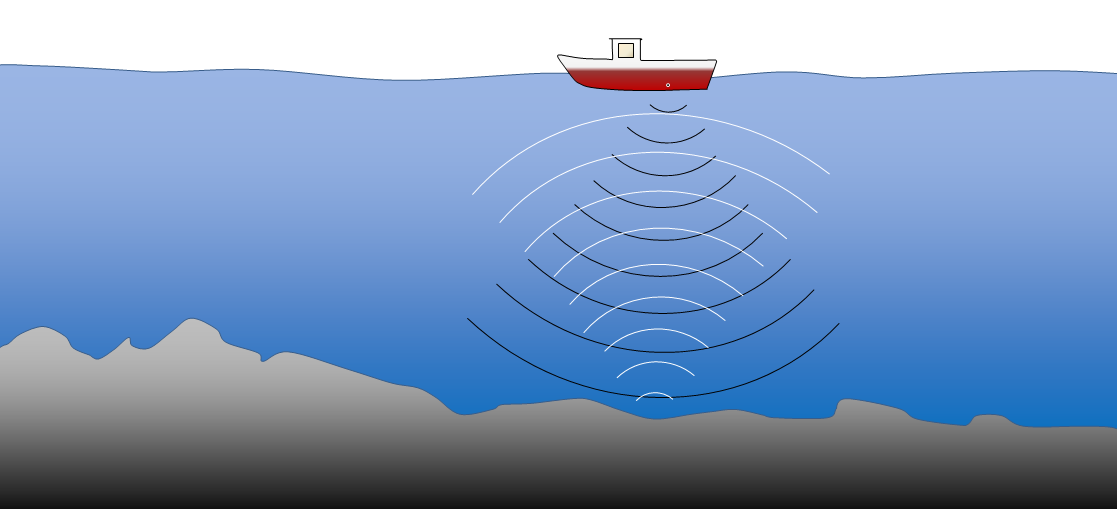
Following development of acoustic depth sounders (Figure 4.10) in the 1920s, the number of depth readings increased by many orders of magnitude, and by the 1930s there was no doubt that major mountain chains ran through all of the world’s oceans. During and after World War II, there was a well-organized campaign to study the oceans, and by 1959, sufficient bathymetric data had been collected to produce detailed maps of all the oceans (Figure 4.11).
_](figures/04-plate-tectonics/figure-4-11.png)
Figure 4.10: A ship-borne acoustic depth sounder. The instrument emits sound (black arcs) that reflects off the sea floor and returns to the surface (white arcs). The time interval between emitting the sound and detecting it on receivers on the ship is proportional to the water depth. Source: Steven Earle (2015) CC BY 4.0 view source
; Basemap after NOAA (2006) Public Domain _[_view source_](https://commons.wikimedia.org/wiki/File:Elevation.jpg)](figures/04-plate-tectonics/figure-4-12.png)
Figure 4.11: Ocean floor bathymetry (and continental topography). Inset (a): the mid-Atlantic ridge, (b): the Newfoundland continental shelf, (c): the Nazca trench adjacent to South America, and (d): the Hawaiian Island chain. Source: Steven Earle (2015) CC BY 4.0 view source; Basemap after NOAA (2006) Public Domain view source
The important physical features of the ocean floor are:
- Extensive linear ridges (commonly in the central parts of the oceans) at depths of 2,000 to 3,000 m (Figure 4.11a)
- Fracture zones perpendicular to the ridges (Figure 4.11a)
- Deep-ocean plains at depths of 4,000 to 5,000 m (Figure 4.11a and d)
- Relatively flat and shallow continental shelves with depths under 500 m (Figure 4.11b)
- Deep trenches (up to 11,000 m deep), most near the continents (Figure 4.11c)
- Seamounts and chains of seamounts (Figure 4.11d)
4.3.2.2 Seismic Reflection Sounding
Seismic reflection sounding involves transmitting high-energy sound bursts and then measuring the echoes with a series of receivers called geophones towed behind a ship. The technique is related to acoustic sounding as described above, however, much more energy is transmitted and the sophistication of the data processing is much greater. As the technique evolved, and the amount of energy was increased, it became possible to see_ through_ the sea-floor sediments and map the bedrock topography and crustal thickness. This allowed sediment thicknesses to be mapped (Figure 4.12).
_](figures/04-plate-tectonics/figure-4-13.jpg)
Figure 4.12: Map of global sediment thickness. Source: NOAA (2003) Public Domain view source
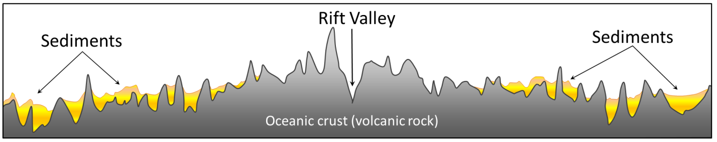
It was soon discovered that although the sediments were up to several 1000s of m thick near the continents, they were relatively thin — or even non-existent — along ocean ridges (Figure 4.13). The seismic studies also showed that the crust is relatively thin under the oceans (5 km to 6 km) compared to the continents (30 km to 60 km) and geologically very consistent, composed almost entirely of basalt.
](figures/04-plate-tectonics/figure-4-14.png)
Figure 4.13: Topographic section at an ocean ridge based on reflection seismic data. Sediments are not thick enough to be detectable near the ridge, but get thicker on either side. The diagram represents approximately 50 km width, and has a 10x vertical exaggeration. Source: Steven Earle (2015) CC BY 4.0 view source
4.3.2.3 Heat Flow Rates
In the early 1950s, Edward Bullard—who spent time at the University of Toronto but is mostly associated with Cambridge University—developed a probe for measuring the flow of heat from the ocean floor. Bullard and colleagues found higher than average heat-flow rates along the ridges, and lower than average rates in trenches. These data were interpreted as evidence of mantle convection, with areas of high heat flow corresponding to upward convection of hot mantle material, and areas of low heat flow corresponding to downward convection.
4.3.2.4 Earthquake Belts
With developments of networks of seismographic stations in the 1950s, it became possible to plot the locations and depths of both major and minor earthquakes with great accuracy. A remarkable correspondence was observed between earthquake locations and both the mid-ocean ridges and the deep ocean trenches. In 1954 Gutenberg and Richter showed that the ocean-ridge earthquakes were all relatively shallow, and confirmed what had first been shown by Benioff in the 1930s, that earthquakes in the vicinity of ocean trenches were both shallow and deep, but that the deeper ones were situated progressively farther inland from the trenches (Figure 4.14).
_](figures/04-plate-tectonics/figure-4-15.png)
Figure 4.14: Aleutian Island subduction zone earthquakes. Left- Map view with earthquakes marked as dots. Red dots are the shallowest earthquakes and blue are the deepest. Quakes get deeper further inland from the trench. Right- Cross-section through a-b. Coloured dots show the depth of earthquakes. Colours correspond to dots in the left figure. Earthquake depth is related to the position of the Pacific plate as it travels beneath the North American plate. Source: Steven Earle (2015) CC BY 4.0 view source
4.3.2.5 Magnetic Stripes on the Sea Floor
In the 1950s, scientists from the Scripps Oceanographic Institute in California persuaded the United States Coast Guard to include magnetometer readings on one of their expeditions to study ocean floor topography. The first comprehensive magnetic data set was compiled in 1958 for an area off the coasts of BC and Washington State. This survey revealed a bewildering pattern of low and high magnetic field intensity in sea-floor rocks (Figure 4.15). When the data were first plotted on a map in 1961, nobody understood them — not even the scientists who collected them. Many 1000s of km of magnetic surveys were conducted over the next several years.
 (adapted from Raff and Mason, 1961)._](figures/04-plate-tectonics/figure-4-16.png)
Figure 4.15: Pattern of sea-floor magnetic field intensity off the west coast of British Columbia and Washington. Black regions have higher than average magnetic field instensity, and white regions have lower than average intensity. Source: Steven Earle (2015) CC BY-SA 4.0, modified after U. S. Geological Survey (n.d.) Public Domain view source (adapted from Raff and Mason, 1961).
The wealth of new data from the oceans began to significantly influence geological thinking in the 1960s. In 1960, Harold Hess from Princeton University, advanced a hypothesis with many of the elements that we now accept as plate tectonics. He maintained some uncertainty about his proposal however, and in order to deflect criticism from mainstream geologists, he labelled it “geopoetry.” In fact, until 1962, Hess didn’t even put his ideas in writing — except internally to the U.S. Navy (which funded his research) — but presented them mostly in lectures and seminars.
Hess proposed that new sea floor was generated from mantle material at the ocean ridges, and that old sea floor was dragged down at the ocean trenches and re-incorporated into the mantle. He suggested that the process was driven by mantle convection currents, rising at the ridges and descending at the trenches (Figure 4.16). He also suggested that the less-dense continental crust did not descend with oceanic crust into trenches, but that colliding landmasses were thrust up to form mountains.
Hess’s hypotheses formed the basis for our ideas on sea-floor spreading and continental drift, but did not go so far as to claim that the crust is made up of separate plates. The Hess model was not roundly criticized, but also not widely accepted, partly because evidence was still lacking.
_](figures/04-plate-tectonics/figure-4-17.png)
Figure 4.16: A representation of Harold Hess’s model for sea-floor spreading and subduction. Source: Steven Earle (2015) CC BY 4.0 view source
Collection of magnetic data from the oceans continued in the early 1960s, but the striped patterns remained unexplained. Some assumed that, as with continental crust, the stripes were related to compositional variations in rock, such as variations in the amount of magnetite. The first real understanding of the significance of the striped anomalies was the interpretation by Fred Vine, a Cambridge graduate student. Vine was examining magnetic data from the Indian Ocean and, like others before him, noted that the magnetic patterns were symmetrical on either side of the ridge.
At the same time, other researchers led by groups in California and New Zealand were studying the phenomenon of reversals in Earth’s magnetic field. They were trying to determine when such reversals had taken place over the past several million years by analyzing the magnetic characteristics of hundreds of samples from basaltic flows. As discussed in Chapter 3, Earth’s magnetic field periodically weakens, then becomes virtually non-existent before becoming re-established with the reverse polarity. During periods of reversed polarity, a compass would point south instead of north.
The time scale of magnetic reversals is irregular. The present “normal” event, known as the Bruhnes magnetic chron, has persisted for about 780,000 years. It was preceded by a 190,000-year reversed event; a 50,000-year normal event known as Jaramillo; and then a 700,000-year reversed event (Figure 3.16).
In a paper published in September 1963, Vine and his PhD supervisor Drummond Matthews proposed that the patterns associated with ridges were related to the magnetic reversals, and that oceanic crust created from cooling basalt during a normal event would have polarity aligned with the present magnetic field, and would produce a positive anomaly (a black stripe on the sea-floor magnetic map). Oceanic crust created during a reversed event would have polarity opposite Earth’s present field and thus produce a negative magnetic anomaly (a white stripe). The same idea had been put forward a few months earlier by Lawrence Morley, of the Geological Survey of Canada. However, Morley’s papers submitted earlier in 1963 to Nature and The Journal of Geophysical Research were rejected. The idea is sometimes referred to as the Vine-Matthews-Morley (VMM) hypothesis.
Vine, Matthews, and Morley were the first to show this type of correspondence between the relative widths of the stripes and the durations of the magnetic reversals. The VMM hypothesis was confirmed within a few years when magnetic data were compiled from spreading ridges around the world. It was shown that the same general magnetic patterns were present straddling each ridge, although the widths of the anomalies varied according to the spreading rates characteristic of the different ridges. It was also shown that the patterns corresponded with the known timeline of Earth’s magnetic field reversals.
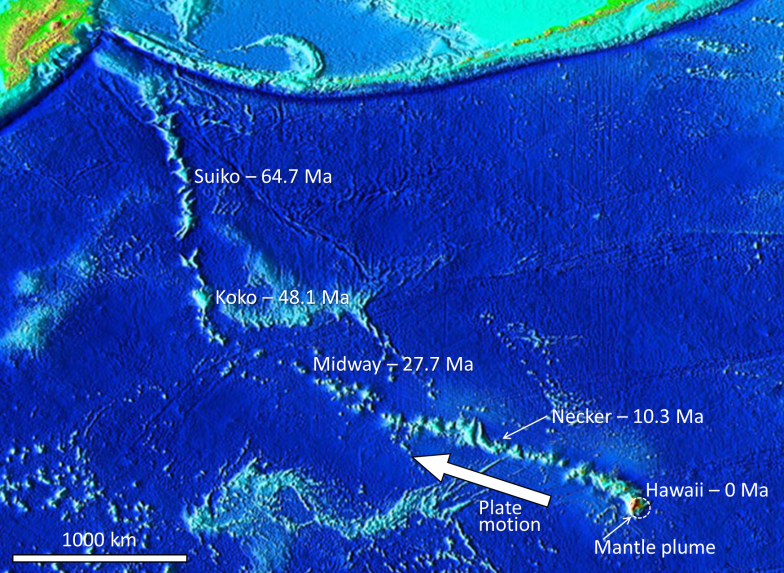
In 1963, J. Tuzo Wilson of the University of Toronto proposed the idea of a mantle plume or hot spot — a place where hot mantle material rises in a stationary and semi-permanent plume, and affects the overlying crust. He based this hypothesis partly on the distribution of the Hawai’ian and Emperor Seamount island chains in the Pacific Ocean (Figure 4.17). The volcanic rock making up these islands becomes progressively younger toward the southeast, culminating in the island of Hawai’i itself, which consists of rock that is almost all younger than 1 Ma.
 Base map from the National Geophysical Data Centre/USGS (2005) Public Domain [view source](http://en.wikipedia.org/wiki/Hotspot_(geology)#/media/File:Hawaii_hotspot.jpg)_](figures/04-plate-tectonics/figure-4-18.png)
Figure 4.17: The ages of the Hawai’ian Islands and the Emperor Seamounts in relation to the location of the Hawai’ian mantle plume. Source: Steven Earle (2015) CC BY 4.0 view source; Base map from the National Geophysical Data Centre/USGS (2005) Public Domain view source
#/media/File:Hawaii_hotspot.jpg)
Wilson suggested that a stationary plume of hot upwelling mantle material is the source of the Hawaiian volcanism, and that the ocean crust of the Pacific Plate is moving toward the northwest over this hot spot. Near the Midway Islands, the chain makes a pronounced change in direction, from northwest-southeast for the Hawai’ian Islands, to nearly north-south for the Emperor Seamounts. This change has been ascribed to a change in direction of the Pacific Plate moving over the stationary mantle plume. An alternative hypothesis is that rather than the Pacific Plate having undergone a sudden change in motion, the plume itself has moved at least 2,000 km south over the period between 81 and 45 Ma (Tarduno et al., 2003).
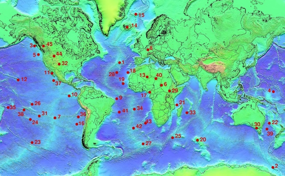
There is evidence of many such mantle plumes around the world (Figure 4.18). Most are within ocean basins, including places like Hawai’i, Iceland, and the Galapagos Islands, but some are under continents. One example is the Yellowstone hot spot in the west-central United States, and another is the one responsible for the Anahim Volcanic Belt in central British Columbia. It is evident that mantle plumes are very long-lived phenomena, lasting for at least tens of millions of years, and possibly for hundreds of millions of years in some cases.
_](figures/04-plate-tectonics/figure-4-19.jpg)
Figure 4.18: Mantle plume locations. Selected Mantle plumes: 1: Azores, 3: Bowie, 5: Cobb, 8: Eifel, 10: Galapagos, 12: Hawai’i, 14: Iceland, 17: Cameroon, 18: Canary, 19: Cape Verde, 35: Samoa, 38: Tahiti, 42: Tristan, 44: Yellowstone, 45: Anahim. Source: Ingo Wölbern (2007) Public Domain view source
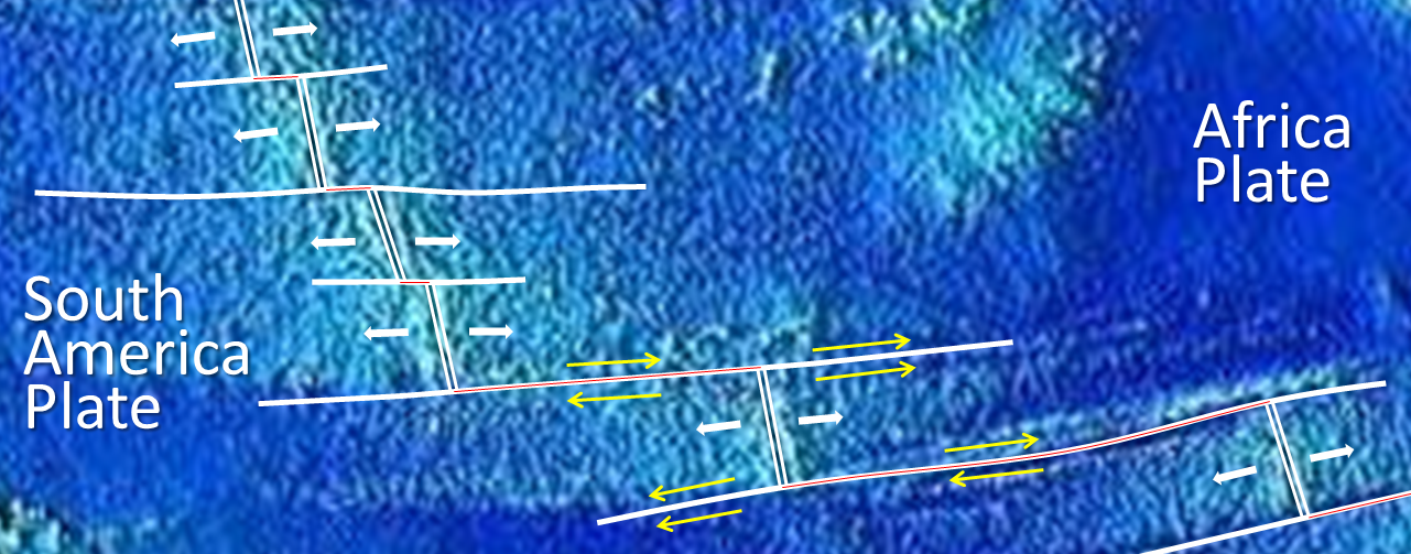
Oceanic spreading ridges appear to be curved features on Earth’s surface, but the ridges are in fact composed of a series of straight-line segments, offset at intervals by faults perpendicular to the ridge (Figure 4.19). In a paper published in 1965, Tuzo Wilson termed these features transform faults.
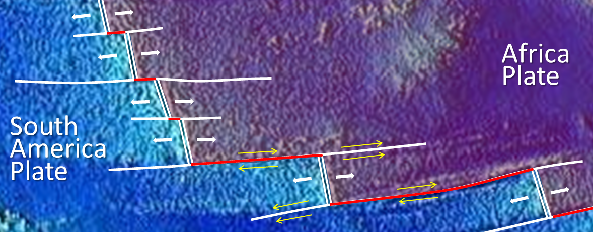_](figures/04-plate-tectonics/figure-4-20.png)
Figure 4.19: Part of the Mid-Atlantic ridge near the equator. Transform faults (red lines) are in between the ridge segments (double white lines), where the yellow arrows (indicating relative plate movement) point in opposite directions. Solid white lines are fracture zones. Source: Steven Earle (2015) CC BY 4.0 view source
In the same 1965 paper, Wilson introduced the idea that the crust can be divided into a series of rigid plates, and is thus responsible for the term plate tectonics.
Exercise: Paper Transform Fault Model
J. Tuzo Wilson used a paper model similar to the one in Figure 4.20 to explain transform faults to his colleagues. To use this model, print Figure 4.20, cut around the outside, and then slice along the line A-B (the fracture zone) with a sharp knife. Fold down the top half where shown, and then pinch together in the middle. Do the same with the bottom half. When you’re done, you should have two folds of paper extending downward as in Figure 4.21.
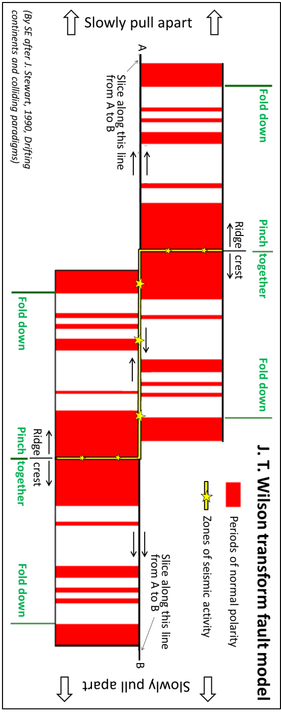, modified after Stewart (1990).](figures/04-plate-tectonics/figure-4-21.png)
Figure 4.20: Transform fault model. Source: Steven Earle (2015) CC BY 4.0 view source, modified after Stewart (1990).
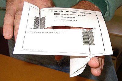_](figures/04-plate-tectonics/figure-4-22.jpg)
Figure 4.21: Use of the transform fault model. Source: Steven Earle (2015) CC BY 4.0 view source
Find someone else to pinch those folds with two fingers just below each ridge crest, and then gently pull apart where shown. As you do, the oceanic crust will emerge from the middle, and you will see that the parts of the fracture zone between the ridge crests will be moving in opposite directions (this is the transform fault) while the parts of the fracture zone outside of the ridge crests will be moving in the same direction. You will also see that the oceanic crust is being magnetized as it forms at the ridge. The magnetic patterns represent the last 2.5 Ma of geological time.
There are other versions of this model available at https://web.viu.ca/earle/transform-model/. For more information see Earle (2004).
4.4 Plates, Plate Motions, and Plate-Boundary Processes
The ideas of continental drift and sea-floor spreading became widely accepted by 1965, and more geologists started thinking in these terms. By the end of 1967, Earth’s surface had been mapped into a series of plates (Figure 4.22). The major plates are Eurasian, Pacific, Indian, Australian, North American, South American, African, and Antarctic plates. There are also numerous small plates (e.g., Juan de Fuca, Nazca, Scotia, Philippine, Caribbean), and many very small plates or sub-plates. The Juan de Fuca Plate is actually three separate plates (Gorda, Juan de Fuca, and Explorer), all moving in the same general direction but at slightly different rates.
_](figures/04-plate-tectonics/figure-4-23.gif)
Figure 4.22: A detailed map of Earth’s tectonic plates. Click on the map to enlarge._ Source: Paul Lowman and Jacob Yates, NASA Goddard Space Flight Center (2002) Public Domain view source_
Plate motions can be tracked using Global Positioning System (GPS) data from different locations on Earth’s surface. Rates of motions of the major plates range from less than 1 cm/y to more than 10 cm/y. The Pacific Plate is the fastest, moving at more than 10 cm/y in some areas, followed by the Australian and Nazca Plates. The North American Plate is one of the slowest, averaging ~1 cm/y in the south up to almost 4 cm/y in the north.
Plates move as rigid bodies, so it may seem surprising that the North American Plate can be moving at different rates in different places. The explanation is that plates rotate as they move; the North American Plate, for example, rotates counter-clockwise, while the Eurasian Plate rotates clockwise.
Boundaries between the plates are of three types: __divergent (__moving apart)_, ___convergent __(moving together), and transform (moving side by side). The plates are made up of crust and lithospheric mantle (Figure 4.23). Even though the plates are in constant motion, and move in different directions, there is never a significant amount of space between them. Plates move along the lithosphere-asthenosphere boundary, because the asthenosphere is relatively weak. It deforms as the plates move, rather than locking them in place.
_](figures/04-plate-tectonics/figure-4-24.png)
Figure 4.23: The crust and upper mantle. Tectonic plates consist of lithosphere, which includes the crust and the lithospheric (rigid) part of the mantle. Source: Steven Earle (2015) CC BY 4.0 view source
At spreading centres, the lithospheric mantle is relatively thin. The upward convective motion of hot mantle material generates temperatures that are too high for the existence of a significant thickness of rigid lithosphere at the same time that the plates are falling away from each other (Figure 4.16).
The fact that plates include both crustal material and lithospheric mantle material makes it possible for a single plate to be include both oceanic and continental crust. The North American Plate includes most of North America, plus half of the northern Atlantic Ocean. Similarly the South American Plate extends across the western part of the southern Atlantic Ocean, while the European and African plates each include part of the eastern Atlantic Ocean. The Pacific Plate is almost entirely oceanic, but it does include the part of California west of the San Andreas Fault.
4.4.1 Divergent Boundaries
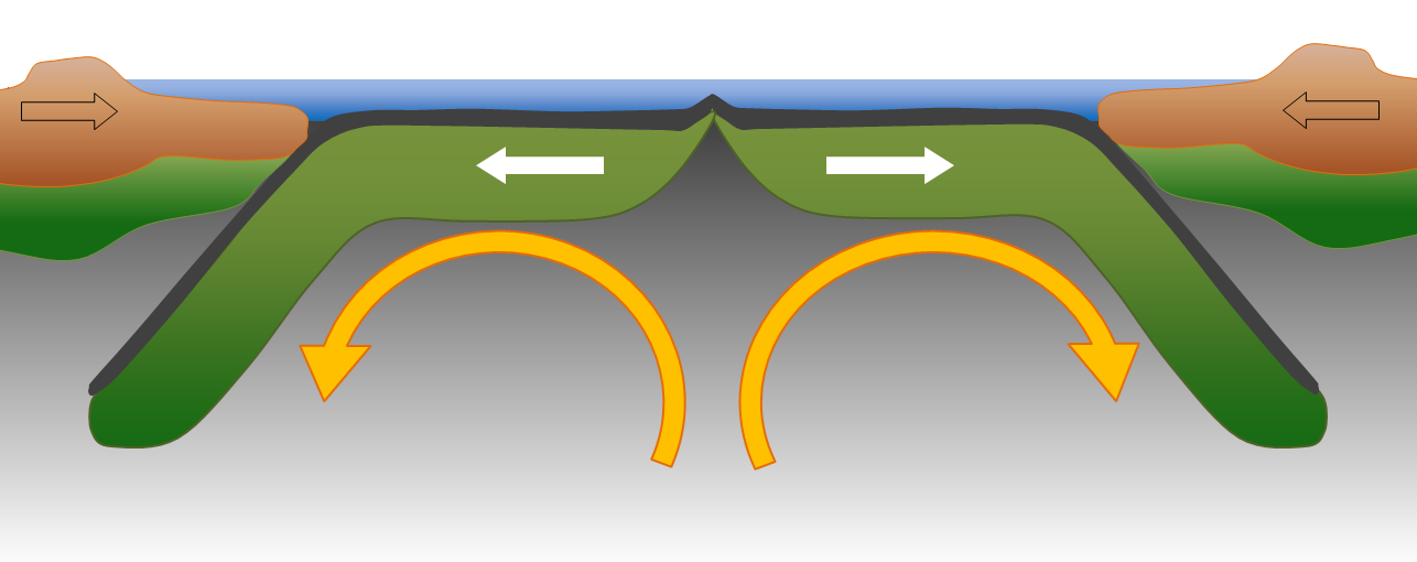
Divergent boundaries are spreading boundaries, where new oceanic crust is created from magma derived from partial melting of the mantle. The partial melting happens when hot mantle rock is moved from deep within Earth where pressures are too high for it to be liquid, to shallower depths where the pressure is much lower (Figure 4.24, bottom left).
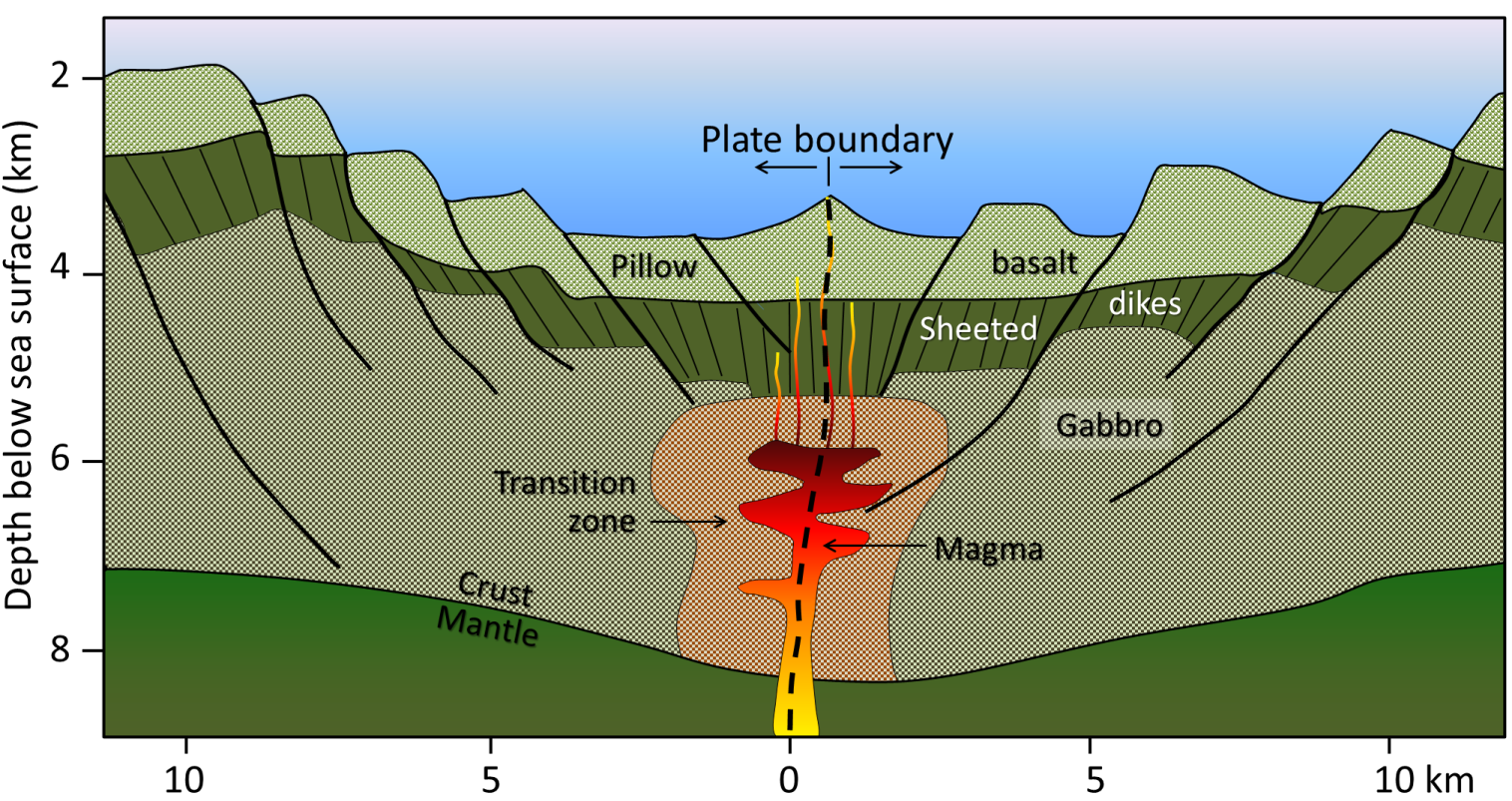
The triangular zone of partial melting near the ridge crest is approximately 60 km thick and the proportion of magma is about 10% of the rock volume, thus producing crust that is about 6 km thick once the melt escapes from the rock in which it formed, and ascends. Most divergent boundaries are located in the oceans, and the crustal material created at a spreading boundary is always oceanic in character; in other words, it is mafic igneous rock (basalt or gabbro, with minerals rich in iron and magnesium). Spreading rates vary considerably, from 1 cm/y to 3 cm/y in the Atlantic, to between 6 cm/y and 10 cm/y in the Pacific. Some of the processes taking place in this setting include (Figure 4.24, top):
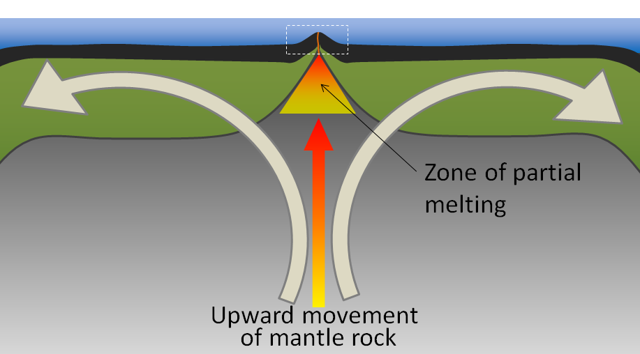; Top- Steven Earle (2015) CC BY 4.0 [view source](https://opentextbc.ca/geology/wp-content/uploads/sites/110/2015/07/image0492.png) modified after Sinton and Detrick (1992); Lower right- NOAA (1988) Public Domain [view source](https://commons.wikimedia.org/wiki/File:Pillow_basalt_crop_l.jpg)_](figures/04-plate-tectonics/figure-4-25.png)
Figure 4.24: Divergent boundary. Lower left- General processes taking place along divergent boundaries. Top- Expanded view of the white box showing divergent boundary processes and materials. Bottom right- Pillow basalts from the ocean floor of Hawai’i. Source: Lower left- Steven Earle (2015) CC BY 4.0 view source; Top- Steven Earle (2015) CC BY 4.0 view source modified after Sinton and Detrick (1992); Lower right- NOAA (1988) Public Domain view source
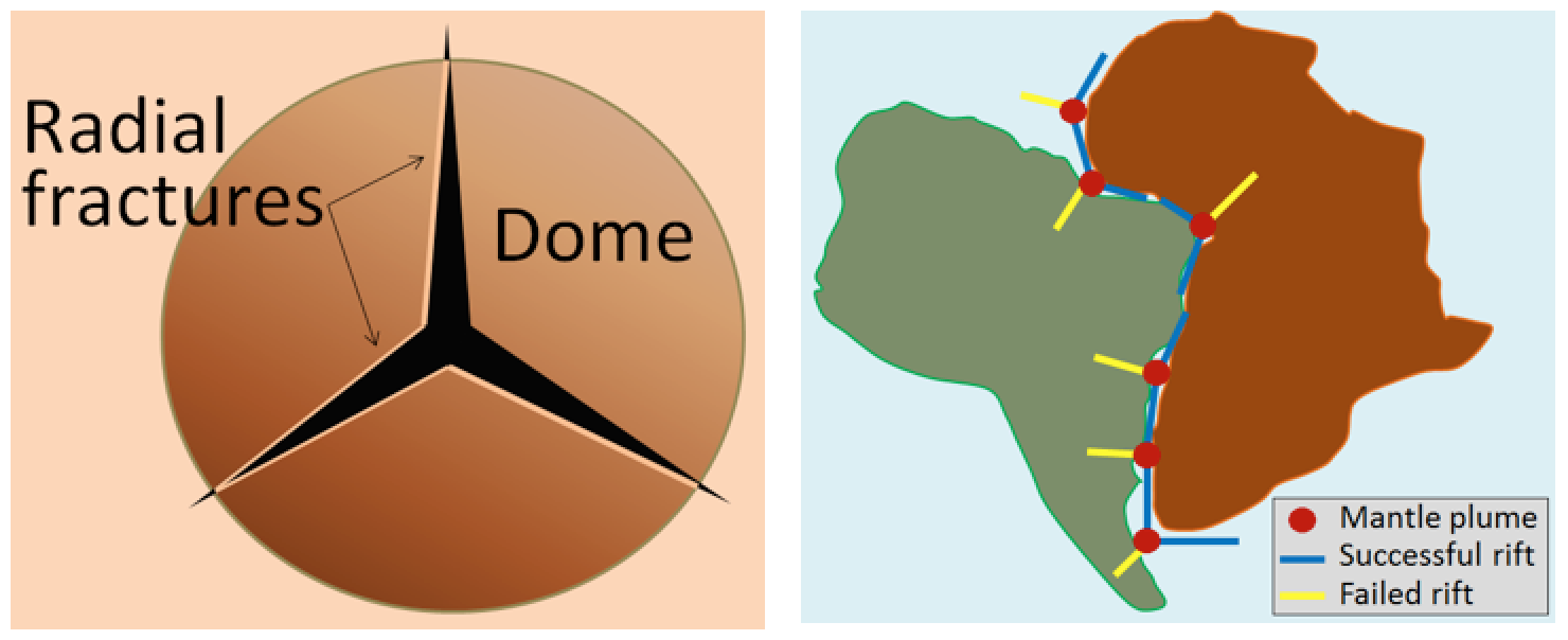
Spreading is thought to start with lithosphere being warped upward into a dome by buoyant material from an underlying mantle plume or series of mantle plumes. The buoyancy of the mantle plume causes the dome to fracture in a radial pattern, with three arms spaced at approximately 120° (Figure 4.25).
](figures/04-plate-tectonics/figure-4-26.png)
Figure 4.25: Depiction of the process of dome and three-part rift formation (left) and of continental rifting between the African and South American parts of Pangea at around 200 Ma (right)_ Source: Steven Earle (2015) CC BY 4.0 _view source
When a series of mantle plumes exists beneath a large continent, the resulting rifts may align and lead to the formation of a rift valley, such as the present-day Great Rift Valley in eastern Africa. This type of valley may eventually develop into a linear sea (such as the present-day Red Sea), and finally into an ocean (such as the Atlantic). It is likely that as many as 20 mantle plumes, many of which still exist, were responsible for the initiation of the rifting of Pangea along what is now the mid-Atlantic ridge (see the Atlantic Ocean mantle plume locations in Figure 4.18).
4.4.2 Convergent Boundaries
Convergent boundaries, where two plates are moving toward each other, are of three types, depending on whether ocean or continental crust is present on either side of the boundary. The types are ocean-ocean, ocean-continent, and continent-continent.
4.4.2.1 Ocean-Ocean Convergent Boundaries
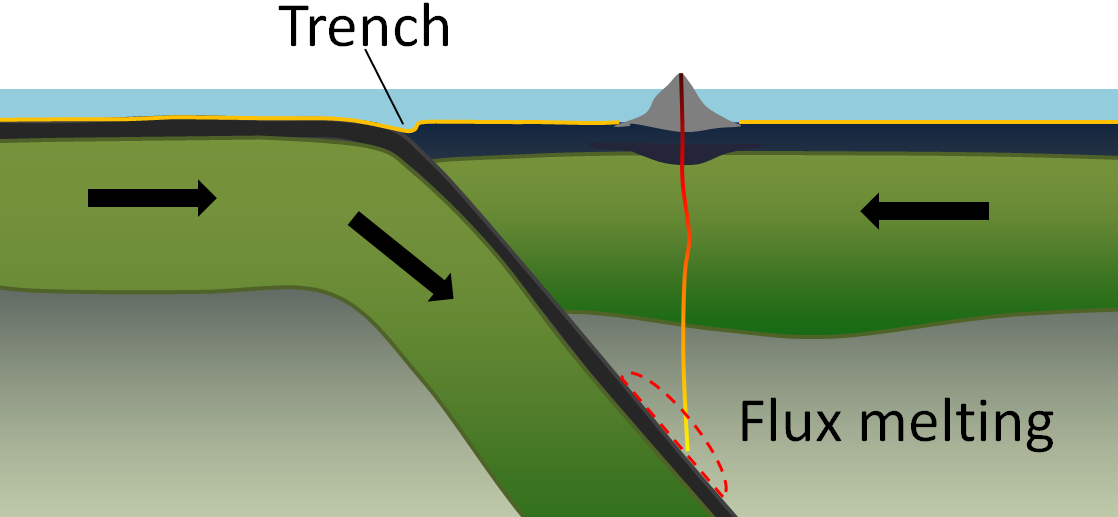
At an ocean-ocean convergent boundary, a plate margin consisting of oceanic crust and lithospheric mantle is subducted_, _or travels beneath, the margin of the plate with which it is colliding (Figure 4.26). Often it is the older and colder plate that is denser and subducts beneath the younger and hotter plate. Ocean trenches commonly form along these boundaries.
_](figures/04-plate-tectonics/figure-4-27.png)
Figure 4.26: Configuration and processes of an ocean-ocean convergent boundary Source: Steven Earle (2015) CC BY 4.0 view source
As the subducting crust is heated and the pressure increases, water is released from within the subducting material. This water comes primarily from alteration of the minerals pyroxene and olivine to serpentine near the spreading ridge shortly after the rock’s formation. The water mixes with the overlying mantle, which lowers the melting point of mantle rocks, causing magma to form. This process is called flux melting or fluid-induced melting.
The newly produced magma, which is lighter than the surrounding mantle rocks, rises through the mantle and sometimes through the overlying oceanic crust to the ocean floor where it creates a chain of volcanic islands known as an island arc. A mature island arc develops into a chain of relatively large islands (such as Japan or Indonesia) as more and more volcanic material is extruded and sedimentary rocks accumulate around the islands. The largest earthquakes occur near the surface where the subducting plate is still cold and strong.
Examples of ocean-ocean convergent zones are subduction of the Pacific Plate south of Alaska (Aleutian Islands) and west of the Philippines, subduction of the Indian Plate south of Indonesia, and subduction of the Atlantic Plate beneath the Caribbean Plate.
4.4.2.2 Ocean-Continent Convergent Boundaries
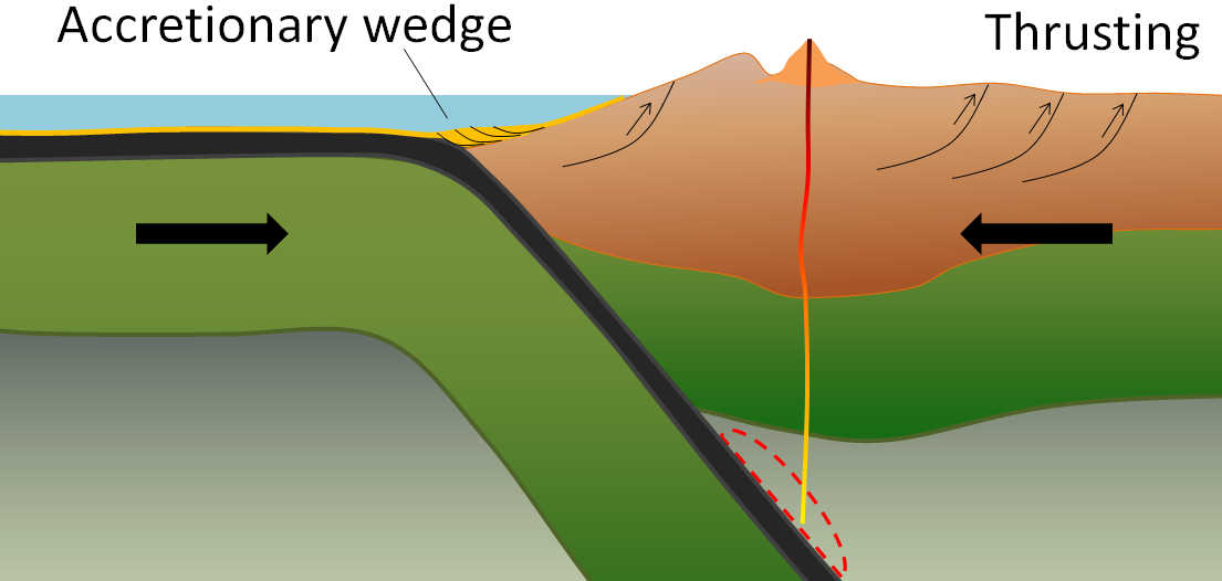
At an ocean-continent convergent boundary, the oceanic plate is subducted beneath the continental plate in the same manner as at an ocean-ocean boundary. Rocks and sediment on the continental slope are thrust up into an accretionary wedge, and compression leads to faults forming within the continental plate (Figure 4.27). The mafic magma produced adjacent to the subduction zone rises to the base of the continental crust and leads to partial melting of the crustal rock. The resulting magma ascends through the crust, producing a mountain chain with many volcanoes.
](figures/04-plate-tectonics/figure-4-28.png)
Figure 4.27: Configuration and processes of an ocean-continent convergent boundary Source: Karla Panchuk (2018) CC BY 4.0, modified after Steven Earle (2015) CC BY 4.0 view source
Examples of ocean-continent convergent boundaries are subduction of the Nazca Plate under South America (which has created the Andes Range) and subduction of the Juan de Fuca Plate under North America (creating the mountains Garibaldi, Baker, St. Helens, Rainier, Hood, and Shasta, collectively known as the Cascade Range).
4.4.2.3 Continent-Continent Convergent Boundary
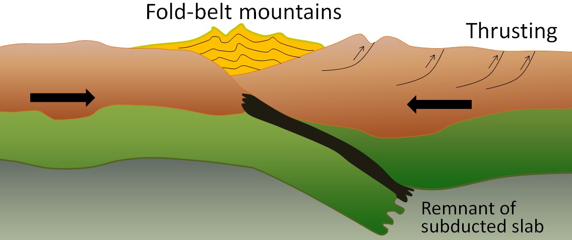
A continent-continent collision occurs when a continent or large island that has been moved along with subducting oceanic crust collides with another continent (Figure 4.28). The colliding continental material will not be subducted because it is not dense enough, but the root of the oceanic plate will eventually break off and sink into the mantle. There is tremendous deformation of the pre-existing continental rocks, and creation of mountains from that rock, as well as from any sediments that had accumulated along the shores of both continental masses, and commonly also from some ocean crust and upper mantle material.
](figures/04-plate-tectonics/figure-4-29.png)
Figure 4.28: Configuration and processes of a continent-continent convergent boundary Source: Steven Earle (2015) CC BY 4.0 view source
Examples of continent-continent convergent boundaries are the collision of the India Plate with the Eurasian Plate, creating the Himalaya Mountains, and the collision of the African Plate with the Eurasian Plate, creating the series of ranges extending from the Alps in Europe to the Zagros Mountains in Iran.
When a subduction zone is jammed shut by a continent-continent collision, plate tectonic stresses that are still present can sometimes cause a new subduction zone to develop outboard of the colliding plate.
4.4.3 Transform Boundaries
Transform boundaries exist where one plate slides past another without producing or destroying crust, except in the special case where the transform boundary has bends and jogs. There will be collisions and divergence on a small scale as the jogs crash into the bends, or open up small windows to deeper crust.
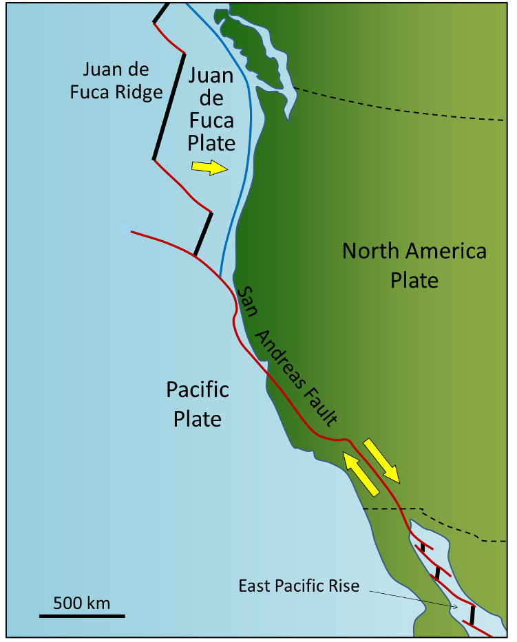
Most transform faults connect segments of mid-ocean ridges and are thus ocean-ocean plate boundaries (Figure 4.19). Some transform faults connect continental parts of plates. An example is the San Andreas Fault, which connects the southern end of the Juan de Fuca Ridge with the northern end of the East Pacific Rise (a ridge) in the Gulf of California (Figures 4.29 and 4.30). The part of California west of the San Andreas Fault and all of Baja California are on the Pacific Plate. But transform faults do not just connect divergent boundaries; the Queen Charlotte Fault connects the north end of the Juan de Fuca Ridge, starting at the north end of Vancouver Island, to the Aleutian subduction zone.
](figures/04-plate-tectonics/figure-4-30.png)
Figure 4.29: The San Andreas Fault extends from the north end of the East Pacific Rise in the Gulf of California to the southern end of the Juan de Fuca Ridge. All of the red lines on this map are transform faults. Source: Steven Earle (2015) CC BY 4.0 view source
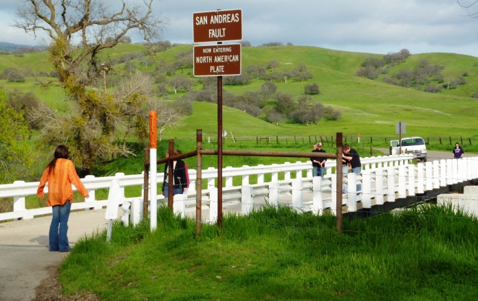](figures/04-plate-tectonics/figure-4-31.jpg)
Figure 4.30: The San Andreas Fault at Parkfield in central California. The person with the orange shirt is standing on the Pacific Plate and the person at the far side of the bridge is on the North American Plate. The bridge is designed to slide on its foundation. Source: Steven Earle (2015) CC BY 4.0 view source
Exercise: A Different Type of Transform Fault
Figure 4.31 shows the Juan de Fuca (JDF) and Explorer plates off the coast of Vancouver Island. The JDF Plate is moving toward the North American Plate at ~ 4.5 cm/y. We think that the Explorer Plate is also moving east, but we don’t know the rate, and there is evidence that it is slower than the JDF Plate.
The boundary between the two plates is the Nootka Fault, which is the location of frequent small-to-medium earthquakes (up to magnitude ~5), as depicted by the red stars. Explain why the Nootka Fault is a transform fault, and show the relative sense of motion along the fault with two small arrows.
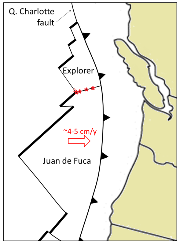_](figures/04-plate-tectonics/figure-4-32.png)
Figure 4.31: Juan de Fuca and Explorer plates separated by the Nootka Fault (marked with red stars). Source: Steven Earle (2015) CC BY 4.0 view source
4.4.4 Plate Tectonics and Supercontinent Cycles
The present continents were once all part of a supercontinent that Alfred Wegener named Pangea (all land). More recent studies of continental matchups and the magnetic ages of ocean-floor rocks have enabled us to reconstruct the history of the break-up of Pangea.
Pangea began to rift apart along a line between Africa and Asia and between North America and South America at around 200 Ma (Figure 4.32). During the same period the Atlantic Ocean began to open up between northern Africa and North America, and India broke away from Antarctica. Between 200 and 150 Ma, rifting started between South America and Africa and between North America and Europe, and India moved north toward Asia. By 80 Ma, Africa had separated from South America, and most of Europe had separated from North America. By 50 Ma, Australia had separated from Antarctica, and shortly after that, India collided with Asia.
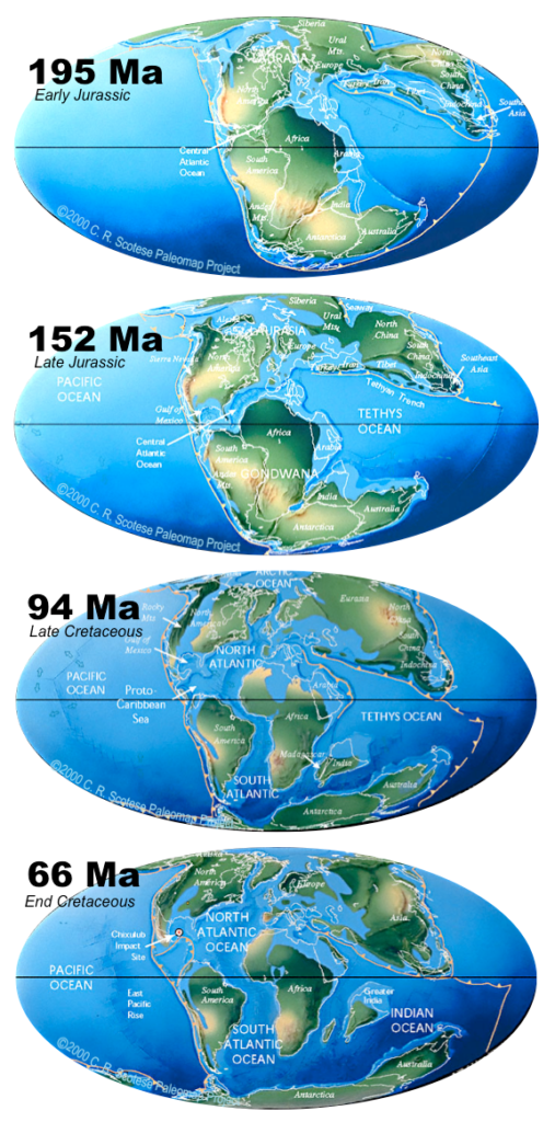
Figure 4.32: Sequence of paleogeographic reconstructions showing the breakup of Pangea. Source: Karla Panchuk (2017) CC BY-NC-SA 4.0. Maps from C. R. Scotese, PALEOMAP Project (www.scotese.com). Click the image for map sources and terms of use.
Within the past few million years, rifting has occurred in the Gulf of Aden and the Red Sea, and also within the Gulf of California. Incipient rifting has begun along the Great Rift Valley of eastern Africa, extending from Ethiopia and Djibouti on the Gulf of Aden (Red Sea) all the way south to Malawi.
Pangea was not the first supercontinent. It was preceded by Pannotia (600 to 540 Ma), Rodinia (1,100 to 750 Ma), and by others before that. In fact, in 1966, Tuzo Wilson proposed that supercontinents are part of an on-going cycle, which we now refer to as a Wilson cycle. In a Wilson cycle, continents break up, and fragments drift apart only to collide again and make a new continent.
At present we are in the stages of a Wilson cycle where fragments are drifting and changing their configuration. North and South America, Europe, and Africa are moving with their respective portions of the Atlantic Ocean. The eastern margins of North and South America and the western margins of Europe and Africa are called passive margins because there is no subduction taking place along them. Because the oceanic crust formed by spreading along the mid-Atlantic ridge is not currently being subducted (except in the Caribbean), the Atlantic Ocean is slowly getting bigger, and the Pacific Ocean is getting smaller.
This situation may not continue for too much longer, however. As the Atlantic Ocean floor gets weighed down around its margins by great thickness of continental sediments, it will be pushed farther and farther into the mantle, and eventually the oceanic lithosphere may break away from the continental lithosphere and begin to subduct (Figure 4.33).
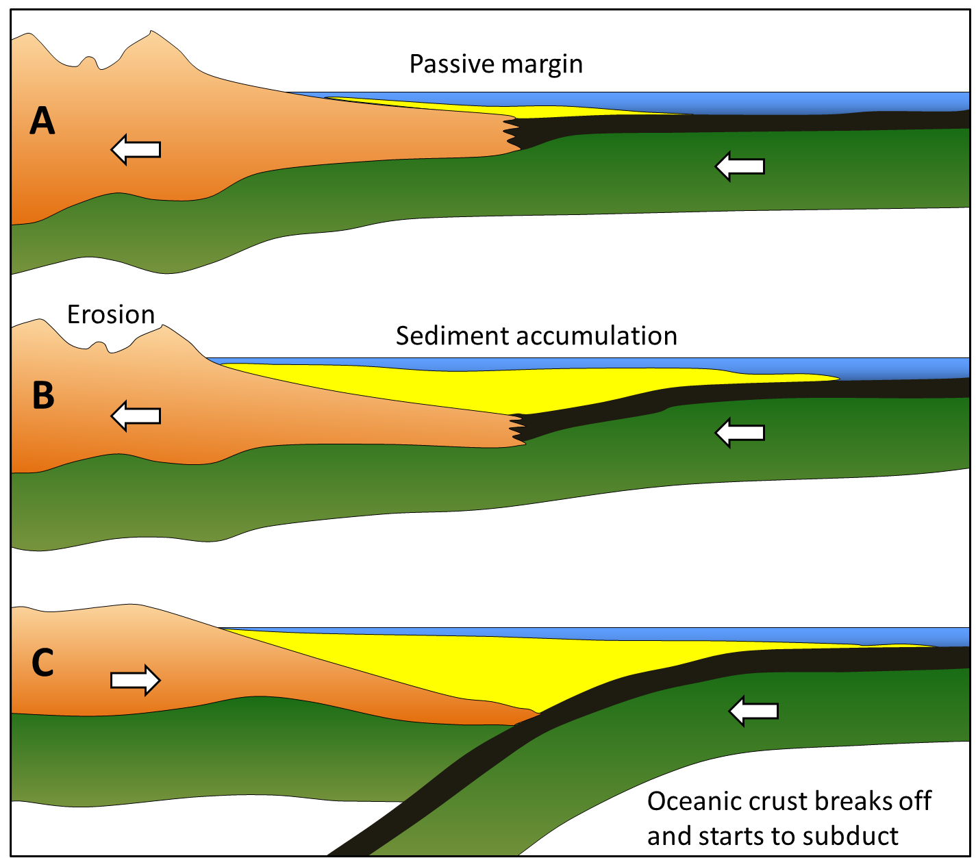_](figures/04-plate-tectonics/figure-4-34.png)
Figure 4.33: Development of a subduction zone at a passive margin. Times A, B, and C are separated by tens of millions of years. Once the oceanic crust breaks off and starts to subduct, the continental crust (North America in this case) may no longer be pushed to the west and could start to move east because the rate of spreading in the Pacific basin is faster than along the Mid-Atlantic Ridge. Source: Steven Earle (2015) CC BY 4.0 view source
A subduction zone will develop, and the oceanic plate will begin to descend under the continent. Once this happens, the continents will no longer continue to move apart because the spreading at the mid-Atlantic ridge will be taken up by subduction. If spreading along the mid-Atlantic ridge continues to be slower than spreading within the Pacific Ocean, the Atlantic Ocean will start to close up, and eventually (in a 100 million years or more) North and South America will collide again with Europe and Africa. If this continues without changing for another few hundred million years, we will be back to where we started, with one supercontinent (Figure 4.34).
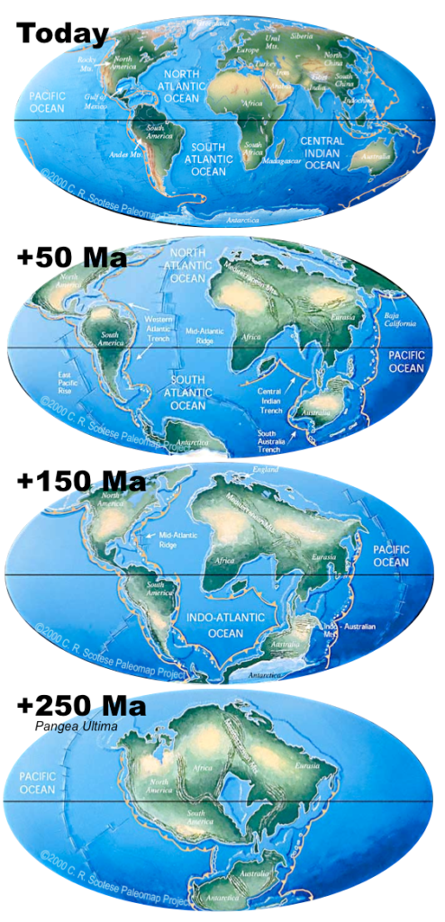
Figure 4.34: Sequence of reconstructions showing the possible future configuration of land masses on Earth at 50, 150, and 250 million years from now. Movements culminate in the formation of a new supercontinent called Pangea Ultima. Source: Karla Panchuk (2017) CC BY-NC-SA 4.0. Maps from C. R. Scotese, PALEOMAP Project (www.scotese.com). Click the image for map sources and terms of use.
There is strong evidence around the margins of the Atlantic Ocean that this process has taken place before. There are roots of ancient mountain belts along the eastern margin of North America, the western margin of Europe, and the north-western margin of Africa, which show that these landmasses once collided with each other to form a mountain chain. The mountain chain might have been as big as the Himalayas.
The apparent line of collision runs between Norway and Sweden, between Scotland and England, through Ireland, through Newfoundland and the Maritimes, through the north-eastern and eastern states, and across the northern end of Florida. When rifting of Pangea started at approximately 200 Ma, the fissuring was along a different line from the line of the earlier collision. This is why some of the mountain chains formed during the earlier collision can be traced from Europe to North America and from Europe to Africa.
It is probably no coincidence that the Atlantic Ocean rift may have occurred in approximately the same place during two separate events several hundred million years apart. The series of hot spots that has been identified in the Atlantic Ocean may also have existed for several hundred million years, and thus may have contributed to rifting in roughly the same place on at least two separate occasions (Figure 4.35).
](figures/04-plate-tectonics/figure-4-36.png)
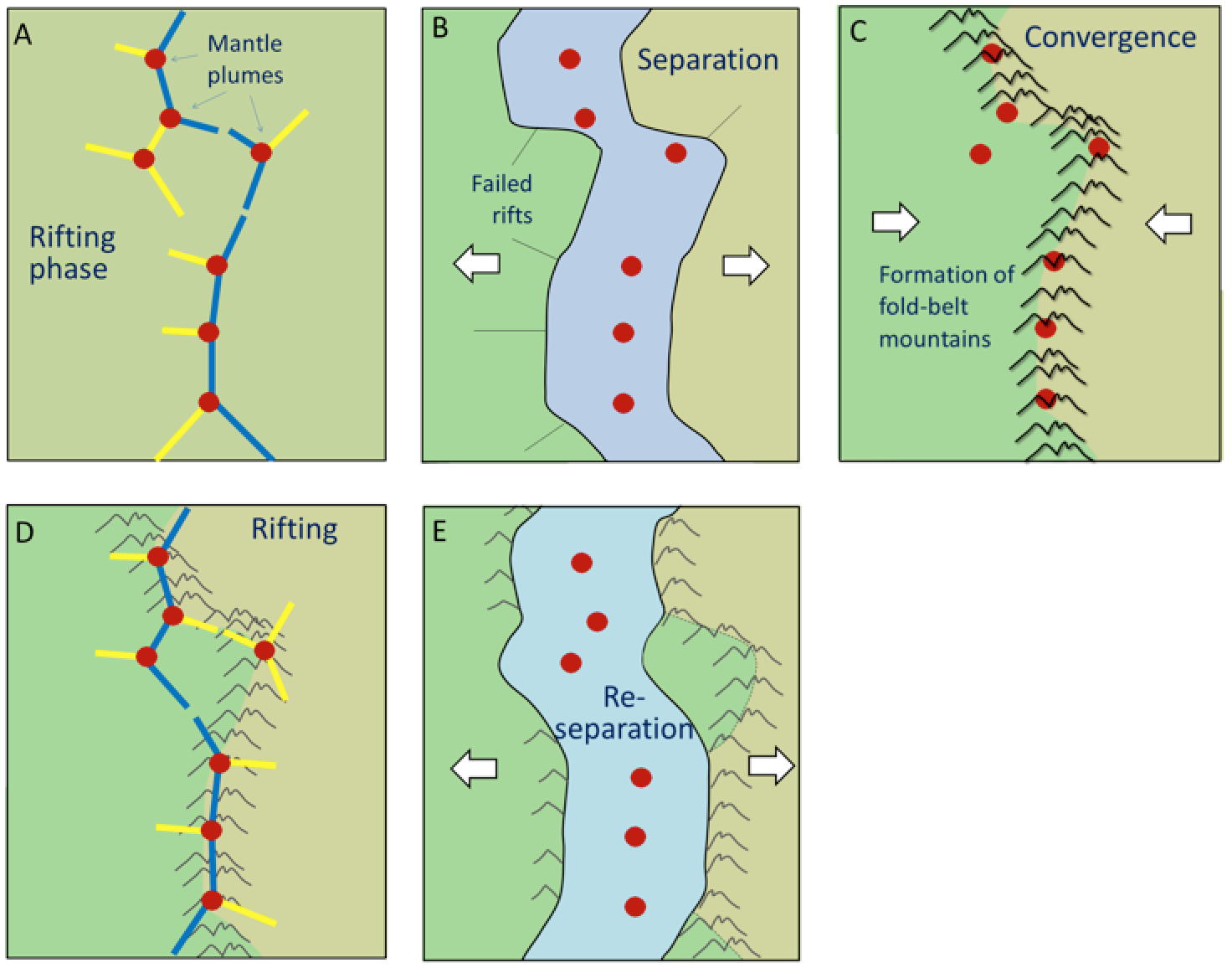
Figure 4.35: A scenario for the Wilson cycle. The cycle starts with continental rifting above a series of mantle plumes (red dots, A). The continents separate (B), and then re-converge some time later, forming a fold-belt mountain chain. Eventually rifting is repeated, possibly because of the same set of mantle plumes (D), but this time the rift is in a different place. Source: Steven Earle (2015) CC BY 4.0 view source
4.5 Mechanisms for Plate Motion
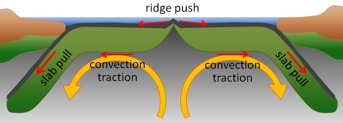
Mantle convection is often said to be critical to plate tectonics. While this is almost certainly so, there is still debate about the actual forces that make the plates move. One side of the argument holds that the plates are only moved by the traction caused by mantle convection, and that friction between the asthenosphere and lithosphere pulls the lithosphere along as the mantle convects. The other side holds that traction plays only a minor role and that ridge-push and slab-pull are more important (Figure 4.36).
Ridge-push refers to gravity causing lithosphere to slide downhill away from the elevated mid-ocean ridges. Slab-pull refers to the weight of subducting slabs dragging the rest of the plate down into the mantle.
_](figures/04-plate-tectonics/figure-4-37.png)
Figure 4.36: Models for plate motion mechanisms. Source: Steven Earle (2015) CC BY 4.0 view source
Kearey and Vine (1996) have listed some compelling arguments in favour of the ridge-push/slab-pull model:
- Plates that are attached to subducting slabs (e.g., Pacific, Australian, and Nazca Plates) move the fastest, and plates that are not (e.g., North American, South American, Eurasian, and African Plates) move significantly slower.
- In order for the traction model to apply, the mantle would have to be moving about five times faster than the plates are moving because the coupling between the partially liquid asthenosphere and the plates is not strong. Such high rates of convection are not supported by geophysical models.
- Although large plates have the potential for much higher convection traction, plate velocity is not related to plate area.
4.6 Summary
The topics covered in this chapter can be summarized as follows:
4.6.1 Alfred Wegener’s Arguments for Plate Tectonics
The evidence for continental drift in the early 20th century included the matching of continental shapes on either side of the Atlantic, and the geological and fossil matchups between continents that are now thousands of kilometres apart.
4.6.2 Global Geological Models of the Early 20th Century
The established theories of global geology were permanentism and contractionism, but neither of these theories was able to explain some of the evidence that supported the idea of continental drift.
4.6.3 Geological Renaissance of the Mid-20th Century
Giant strides were made in understanding Earth during the middle decades of the 20th century, including discovering magnetic evidence of continental drift, mapping the topography of the ocean floor, describing the depth relationships of earthquakes along ocean trenches, measuring heat flow differences in various parts of the ocean floor, and mapping magnetic reversals on the sea floor. By the mid-1960s, the fundamentals of the theory of plate tectonics were in place.
4.6.4 Plates, Plate Motions, and Plate-Boundary Processes
Earth’s lithosphere is made up of over 20 plates that are moving in different directions at rates of between 1 cm/y to greater than 10 cm/y. The three types of plate boundaries are divergent (plates moving apart and new crust forming), convergent (plates moving together and one possibly being subducted), and transform (plates moving side by side). Divergent boundaries form where existing plates are rifted apart, and it is hypothesized that this is caused by a series of mantle plumes. Subduction zones can form where accumulation of sediment at a passive margin leads to separation of oceanic and continental lithosphere. Supercontinents form and break up through these processes.
4.6.5 Mechanisms for Plate Motion
It is widely believed that ridge-push and slab-pull are the main mechanisms for plate motion, as opposed to traction by mantle convection. Mantle convection is a key factor for producing the conditions necessary for ridge-push and slab-pull.
4.7 Chapter Review Questions
List some of the evidence used by Wegener to support his idea of moving continents.
What was the primary weakness in Wegener’s continental drift hypothesis?
How were mountains thought to be formed (a) by contractionists and (b) by permanentists?
How were the trans-Atlantic paleontological matchups explained in the late 19th century?
How did we learn about the topography of the sea floor in the early part of the 20th century?
What evidence from paleomagnetic studies provided support for continental drift?
Which parts of the oceans are the deepest?
Why is there less sediment along ocean ridges than on other parts of the sea floor?
How were the oceanic heat-flow data related to mantle convection?
Describe the spatial distribution of earthquakes at ocean ridges and ocean trenches.
In the model for ocean basins developed by Harold Hess, what happens at oceanic ridges and what happens at oceanic trenches?
What aspect of plate tectonics was not included in the Hess model?
What is a mantle plume and what is its expected lifespan?
Describe the nature of movement at an ocean ridge transform fault (a) between the ridge segments, and (b) outside of ridge segments.
How is it possible for a plate to include both oceanic and continental crust?
What is the likely relationship between mantle plumes and the development of a continental rift?
Why does subduction not take place at a continent-continent convergence zone?
Where are Earth’s most recent sites of continental rifting and creation of new ocean floor?
What geological situation might eventually lead to the generation of a subduction zone at a passive ocean-continent boundary such as the eastern coast of North America?
4.8 Answers to Chapter Review Questions
The evidence used by Wegener to support his idea of moving continents included matching continental shapes and geological features on either side of the Atlantic; common terrestrial fossils in South America, Africa, Australia, and India; and data on the rate of separation between Greenland and Europe.
The primary weakness of Wegener’s theory was that he had no realistic mechanism for making continents move.
Contractionists believed that mountains formed because the crust wrinkled into mountains as Earth cooled and contracted. Permanentists believed that mountains formed by the geosynclinal process.
In the late 19th century the trans-Atlantic paleontological matchups were explained by assuming that there must have been land bridges between the continents at some time in the past.
Prior to 1920, ocean depths were measured by dropping a weighted line over the side of ship. Echo sounding techniques were developed at around that time and greatly facilitated the measurement of ocean depths.
Paleomagnetic studies showed that old rocks on the continents indicated different locations for magnetic north than the position of magnetic north today. They also showed that the difference in pole position from data on different continents increased progressively for older and older rocks. This implied that either Earth had more than one magnetic pole moving around, or that the continents had moved.
Trenches associated with subduction zones are the deepest parts of the oceans.
The ocean ridge areas are the youngest parts of the sea floor and thus there hasn’t been time for much sediment to accumulate.
It was (and still is) thought that high heat flow exists where mantle convection cells are moving hot rock from the lower mantle toward the surface, and that low heat flow exists where there is downward movement of mantle rock.
Earthquakes are consistently shallow and relatively small at ocean ridges. At ocean trenches earthquakes become increasingly deep in the direction that the subducting plate is moving.
In the Hess model new crust was formed at ocean ridges. Crust was recycled back into the mantle at the trenches.
Hess’s model did not include the concept of tectonic plates.
A mantle plume is a column of hot rock (not magma) that ascends toward the surface from the lower mantle. Mantle plumes last tens of millions of years to hundreds of millions of years.
- Between the ridge segments there is movement in opposite directions along a transform fault. (b) Outside of the ridge segments the two plates are moving in the same direction and likely at about the same rate. These regions are known as fracture zones.
Tectonic plates are made up of crust and the lithospheric (rigid) part of the underlying mantle. The mantle part ensures that the very different oceanic and continental crust sections of a plate can act as one unit.
A mantle plume beneath a continent can cause the crust to form a dome that might eventually split open. Several mantle plumes along a line within a continent could lead to rifting.
Subduction does not take place at a continent-continent convergent zone because neither plate is dense enough to sink into the mantle.
Continental rifting is taking place along the East Africa Rift, and sea floor has recently been created in the Red Sea and also in the Gulf of California.
The accumulation of sediment at a passive ocean-continent boundary will lead to the depression of the lithosphere and could eventually result in the separation of the oceanic and continental parts of the plate and the beginning of subduction.
4.9 References
Wegener, A. (1920). Die Entstehung der Kontinente und Ozeane. Braunschweig, Germany: Friedr. Vieweg & Sohn. Full text at Project Gutenberg
Thordarson, T., and Larsen, G. (2007) Volcanism in Iceland in historical time: Volcano types, eruption styles and eruptive history. Journal of Geodynamics 43, 118–152. Full text
Ingersoll, E. (1919). Land-Bridges Across the Oceans. In The Encyclopedia Americana (Vol. XVI, pp. 692-694). New York, NY: Encyclopedia Americana Corporation. Full text
Kuenen, P. H. (1937) The negative isostatic anomalies in the East Indies (with Experiments). Leidse Geologische Mededelingen 8(2), 169-214. Full text
Earle, S. (2004). A simple paper model of a transform fault at a spreading ridge. Journal of Geoscience Education 52, 391-392.
Raff, A., & Mason, R. (1961) Magnetic survey off the west coast of North America, 40˚ N to 52˚ N latitude. Geological Society of America Bulletin 72, 267-270.
Stewart, J. A. (1990). Drifting continents and colliding paradigms. Bloomington IN: Indiana University Press.
Tarduno, J. A., Duncan, R. A., Scholl, D. W., Cottrell, R. D., Steinberger, B., Thordarson, T., Kerr, B. C., Neal, C. R., Frey, F. A., Torii, M., and Carvallo, C. (2003). The Emperor Seamounts: Southward Motion of the Hawaiian Hotspot Plume in Earth’s Mantle. Science 301(5636), 1064–1069. DOI:10.1126/science.1086442
Wilson, J. T. (1965). A new class of faults and their bearing on continental drift. Nature 207, 343-347.
Sinton, J. M., and Detrick, R. S. (1992). Mid-Ocean Ridge Magma Chambers. Journal of Geophysical Research 97(B1), 197-216.
Kearey, P., & Vine, F. (1996). Global Tectonics (2nd E.). Oxford: Blackwell Science Ltd.
Ted Irving later set up a paleomagnetic lab at the Geological Survey of Canada in Sidney BC, and did important work on understanding the geology of western North America.↩︎