Chapter 12 Earthquakes
Adapted from Physical Geology, First University of Saskatchewan Edition (Karla Panchuk) and Physical Geology (Steven Earle)
. Click the image for more attributions._](figures/12-earthquakes/figure-12-1.png)
Figure 12.1: Demolition of a structure damaged when an earthquake of magnitude 6.3 struck Christchurch, New Zealand on February 22, 2011. Many structures had already sustained damage from an earthquake that struck six months earlier, in September of 2010. Collapsing structures and falling debris accounted for most of the 185 deaths. Source: Karla Panchuk (2017) CC BY-SA 4.0. Photograph: Terry Philpott (2012) CC BY-NC 2.0 view source. Click the image for more attributions.
Learning Objectives
After reading this chapter, and answering the review questions at the end, you should be able to:
- Explain how elastic deformation of Earth’s crust results in earthquakes.
- Describe how the main shock and immediate aftershocks define the rupture surface of an earthquake, and explain how the transfer of stress to other parts of a fault is related to aftershocks.
- Explain the process of episodic tremor and slip.
- Explain how plate tectonic setting affects where earthquakes occur.
- Distinguish between an earthquake’s magnitude and its intensity, and explain how these are determined.
- Describe the hazards caused by earthquakes, including ground shaking, fires, slope failures, liquefaction, and tsunami.
- Explain how the risk of an earthquake can be assessed, and describe steps that governments and individuals can take to minimize the impacts of earthquakes.
12.0.1 Why Study Earthquakes?
On the morning of June 23, 1946, a magnitude 7.3 earthquake struck Vancouver Island. It caused substantial damage to structures, including the school shown in Figure 12.2, and resulting in one fatality. The shaking was so violent that the seismograph measuring the earthquake in Victoria was broken a few seconds after the earthquake started. Even if the seismograph had survived, it was not sensitive enough to provide sufficiently detailed information about local earthquakes, and was unable to record some of them at all. There was only one monitoring station in British Columbia, so while it was possible to determine how far away the earthquake was from the station, geologists were not able to say in which direction. In 1955, Canadian seismologist W. G. Milne wrote that “the 1946 earthquake indicated in a very forceful manner the need for better instruments for the study of earthquakes in British Columbia.” A network of improved instruments was established as a direct result of the earthquake.
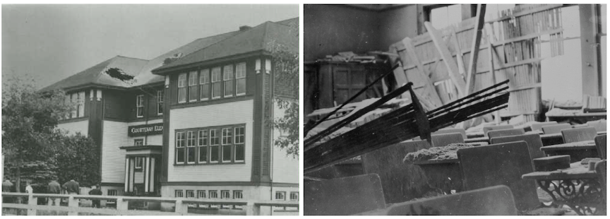
Figure 12.2: Damage to an elementary school in Courtenay, British Columbia after a magnitude 7.3 earthquake on Sunday, June 23, 1946. Left: A hole left after the chimney collapsed through the roof. Right: Damage inside the school. In addition to damaging structures, the earthquake triggered numerous slope failures. Source: Photographs courtesy of Earthquakes Canada. Click the image for image sources and terms of use.
Time and time again earthquakes have caused massive damage and many, many casualties. Recording earthquakes and determining their location of origin is important for establishing what geological conditions are responsible for the earthquakes, and understanding the risk they pose. After new, more sensitive instruments were installed at the Dominion Astrophysical Observatory in Victoria, geologists quickly learned that they had underestimated earthquake activity in the area. Between June of 1948 and August of 1951, 224 local earthquakes were recorded!
By studying earthquakes, geoscientists and engineers are making progress toward learning how to minimize earthquake damage, and how to reduce the number of people affected by earthquakes. This knowledge can be communicated to governments, so they are aware of what is needed to keep the population safe. It can also be communicated to individuals, so they know what to expect and do in the event of an earthquake, and can be adequately prepared with emergency supplies.
12.0.1.0.0.1 Additional Resources
Lamontagne, M., Halchuk, S., Cassidy, J. F., and Rogers, G. C (2008) Significant Canadian Earthquakes of the Period 1600 - 2008. Seismological Research Letters 79(2), 211 - 223. doi: 10.1785/gssrl.79.2.211 Read the paper
Detailed description of the effects of the 1946 earthquake: Hodgson, E. A. (1946). British Columbia Earthquake, June 23, 1946. The Journal of the Royal Astronomical Society of Canada XL(8), 285 - 319. Read the paper
12.1 What is an Earthquake?
12.1.1 Earthquake Shaking Comes from Elastic Deformation
Earthquakes occur when rock ruptures (breaks), causing rocks on one side of a fault to move relative to the rocks on the other side. Although motion along a fault is part of what happens when an earthquake occurs, rocks grinding past each other is not what creates the shaking. In fact, it could be said that the earthquake happens _after _rocks have undergone most of the displacement. Consider this: if rocks slide a few centimetres or even metres along a fault, would that motion alone explain the incredible damage caused by some earthquakes? If you were in a car that suddenly accelerated then stopped, you would feel a jolt. But earthquakes are not a single jolt. Buildings can swing back and forth until they shake themselves to pieces, train tracks can buckle and twist into s-shapes, and roads can roll up and down like waves on the ocean. During an earthquake, rock is not only slipping. It is also vibrating like a plucked guitar string.
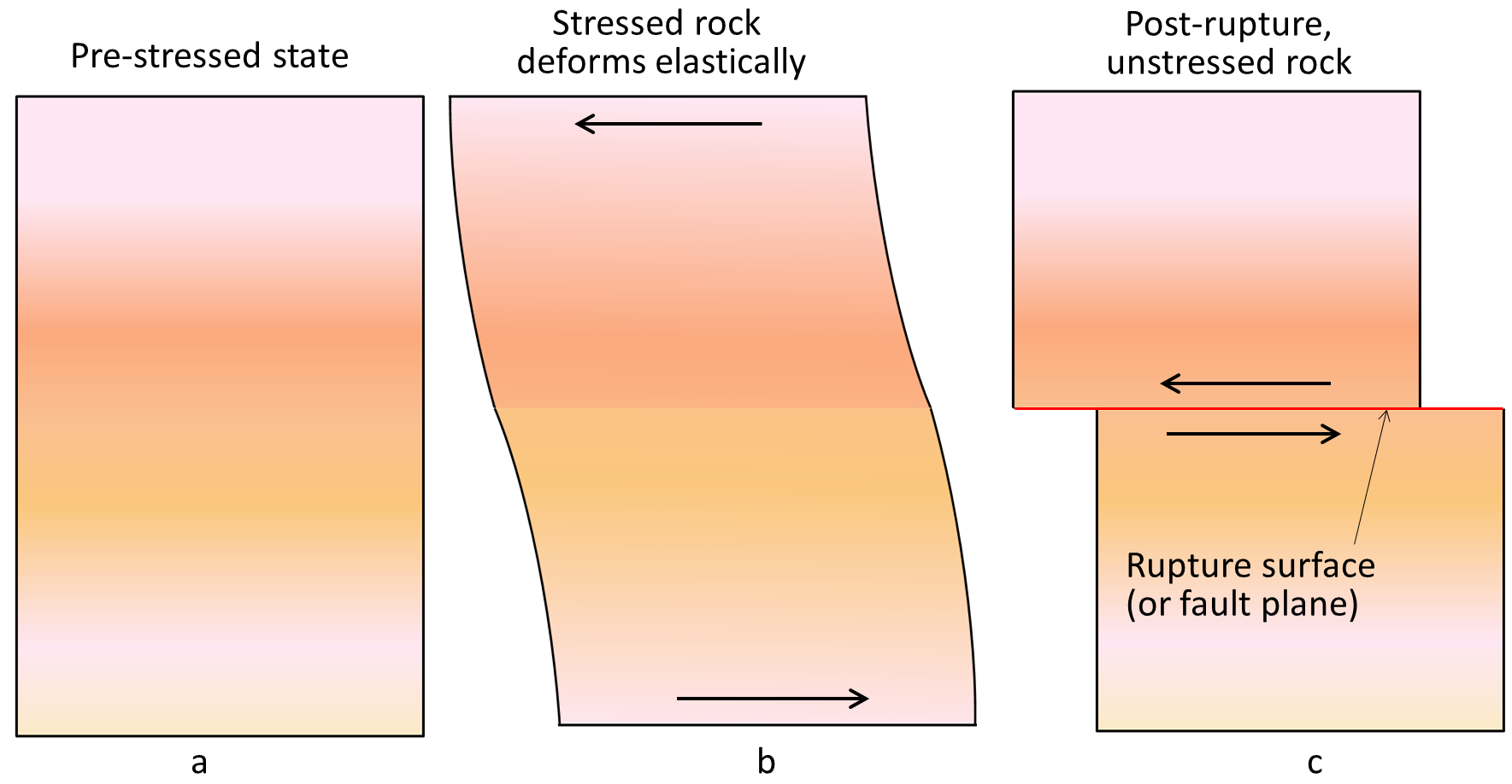
Rocks might seem rigid, but when stress is applied they may stretch. If there hasn’t been too much stretching, a rock will snap back to its original shape once the stress is removed. Deformation that is reversible is called elastic deformation. Rocks that are stressed beyond their ability to stretch can rupture, allowing the rest of the rock to snap back to its original shape. The snapping back of the rock returning to its original shape causes the rock to vibrate, and this is what causes the shaking during an earthquake. The snapping back is called elastic rebound.
Figure 12.3 (top) shows this sequence of events. Stress is applied to a rock and deforms it. The deformed rock ruptures, forming a fault. After rupturing, the rock above and below the fault snaps back to the shape it had before deformation.
._](figures/12-earthquakes/figure-12-3.png)
Figure 12.3: Elastic deformation, rupture, and elastic rebound. Top: Stress applied to a rock causes it to deform by stretching. When the stress becomes too much for the rock, it ruptures, forming a fault. The rock snaps back to its original shape in a process called elastic rebound. Bottom: On an existing fault, asperities keep rocks on either side of the fault from sliding. Stress deforms the rock until the asperities break, releasing the stress, and causing the rocks to spring back to their original shape. Source: Karla Panchuk (2017) CC BY 4.0. Modified after Steven Earle (2015) CC BY 4.0 view original.
Ruptures can also occur along pre-existing faults (Figure 12.3, bottom). The rocks on either side of the fault are locked together because bumps along the fault, called asperities, prevent the rocks from moving relative to each other. When the stress is great enough to break the asperities, the rocks on either side of the fault can slide again. While the rocks are locked together, stress can cause elastic deformation. When asperities break and release the stress, the rocks undergo elastic rebound and return to their original shape.
12.1.2 Rupture Surfaces Are Where the Action Happens
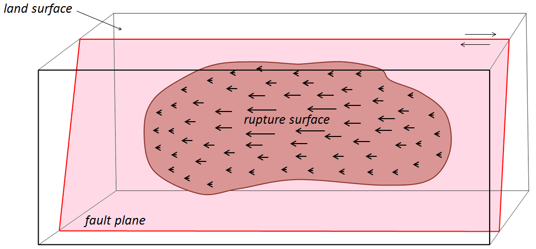
Images like 12.3 are useful for illustrating elastic deformation and rupture, but they can be misleading. The rupture that happens doesn’t occur as in 12.3, with the block being ruptured through and through. The rupture and displacement only happen along a subsection of a fault, called the rupture surface. In Figure 12.4, the rupture surface is the dark pink patch. It takes up only a part of the fault plane (lighter pink). The fault plane represents the surface where the fault exists, and where ruptures have happened in the past. Although the fault plane is drawn as being flat in Figure 12.4, faults are not actually perfectly flat.
The location on the fault plane where the rupture happens is called the hypocentre or focus of the earthquake (Figure 12.4, right). The location on Earth’s surface immediately above the hypocentre is the epicentre of the earthquake.
. Right: Karla Panchuk (2017) CC BY 4.0.<br>_](figures/12-earthquakes/figure-12-4.png)
Figure 12.4: Rupture surface (dark pink), on a fault plane (light pink). The diagram represents a part of the crust that may be tens or hundreds of kilometres long. The rupture surface is the part of the fault plane along which displacement occurred. Left: In this example, the near side of the fault is moving to the left, and the lengths of the arrows within the rupture surface represent relative amounts of displacement. Coloured arrows represent propagation of failure on a rupture surface. In this case, the failure starts at the dark blue heavy arrow and propagates outward, reaching the left side first (green arrows) and the right side last (yellow arrows). Right: An earthquake’s location can be described in terms of its hypocentre (or focus), the location on the fault plane where the rupture happens, or in terms of its epicentre (red star), the location above the hypocentre. Source: Left: Steven Earle (2015) CC BY 4.0 view source. Right: Karla Panchuk (2017) CC BY 4.0.
Within the rupture surface, the amount of displacement varies. In Figure 12.4, the larger arrows indicate where there has been more displacement, and the smaller arrows where there has been less. Beyond the edge of the rupture surface there is no displacement at all. Notice that this particular rupture surface doesn’t even extend to the land surface of the diagram.
The size of a rupture surface and the amount of displacement along it will depend on a number of factors, including the type and strength of the rock, and the degree to which the rock was stressed beforehand. The magnitude of an earthquake will depend on the size of the rupture surface and the amount of displacement.
A rupture doesn’t occur all at once along a rupture surface. It starts at a single point and spreads rapidly from there. Figure 12.4 illustrates a case where rupturing starts at the heavy blue arrow in the middle, then continues through the lighter blue arrows. The rupture spreads to the left side (green arrows), then the right (yellow arrows).
Depending on the extent of the rupture surface, the propagation of failures (incremental ruptures contributing to making the final rupture surface) from the point of initiation is typically completed within seconds to several tens of seconds. The initiation point isn’t necessarily in the centre of the rupture surface; it may be close to one end, near the top, or near the bottom.
12.1.3 Shifting Stress Causes Foreshocks and Aftershocks
Earthquakes don’t usually occur in isolation. There is often a sequence in which smaller earthquakes occur prior to a larger one, and then progressively smaller earthquakes occur after. The largest earthquake in the series is the mainshock. The smaller ones that come before are foreshocks, and the smaller ones that come after are aftershocks. These descriptions are relative, so it can be necessary to reclassify an earthquake. For example, the strongest earthquake in a series is classified as the mainshock, but if another even bigger one comes after it, the bigger one is called the mainshock, and the earlier one is reclassified as an aftershock.
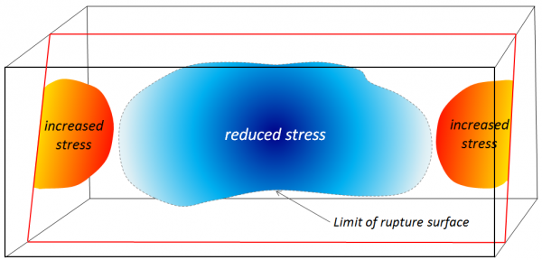
A rupture surface does not fail all at once. A rupture in one place leads to another, which leads to another. Aftershocks and foreshocks represent the same thing, except on a much larger scale. The rupture illustrated in Figure 12.4 reduced stress in one area, but in doing so, transferred stress to others (Figure 12.5). Imagine a frayed rope breaking strand by strand. When a strand breaks, the tension on that strand is released, but the remaining strands must still hold up the same amount of weight. If another strand breaks under the increased burden, the remaining strands have an even greater burden than before. In the same way that the stress causes one strand after another to fail, a rupture can trigger subsequent ruptures nearby.
._](figures/12-earthquakes/figure-12-5.png)
Figure 12.5: Stress changes related to an earthquake. Stress decreases in the area of the rupture surface, but increases on adjacent parts of the fault. Source: Steven Earle (2015) CC BY 4.0 view source.
Numerous aftershocks were associated with the magnitude 7.8 earthquake that struck Haida Gwaii in October of 2012 (Figure 12.6; mainshock in red, aftershocks in white). Some of the stress released by the mainshock was transferred to other nearby parts of the fault, and contributed to a cascade of smaller ruptures. But stress transfer need not be restricted to the fault along which an earthquake happened. It will affect the rocks in general around the site of the earthquake and may lead to increased stress on other faults in the region. The aftershocks from the Haida Gwaii earthquake are scattered rather than located only on the main faults.
. Subduction zone after Wang et al. (2015). Click the image for more attributions._](figures/12-earthquakes/figure-12-6.png)
Figure 12.6: Magnitude 7.8 Haida Gwaii earthquake and aftershocks. Mainshock (red circle marks the epicentre) occurred on October 28th, 2012. Aftershocks are for the period from October 28th to November 10th of 2012. Although the epicentre is near a transform boundary, the rupture was influenced more by compression related to the subduction zone. Source: Karla Panchuk (2017) CC BY 4.0. Base map with epicentres from the U. S. Geological Survey Latest Earthquakes tool view interactive map. Subduction zone after Wang et al. (2015). Click the image for more attributions.
The effects of stress transfer may not show immediately. Aftershocks can be delayed for hours, days, weeks, or even years. Because stress transfer affects a region, not just a single fault, and because there can be delays between the event that transferred stress and the one that was triggered by the transfer, it can sometimes be hard to be know whether one earthquake is actually associated with another, and whether a foreshock or aftershock should be assigned to a particular mainshock.
12.1.4 Episodic Tremor and Slip
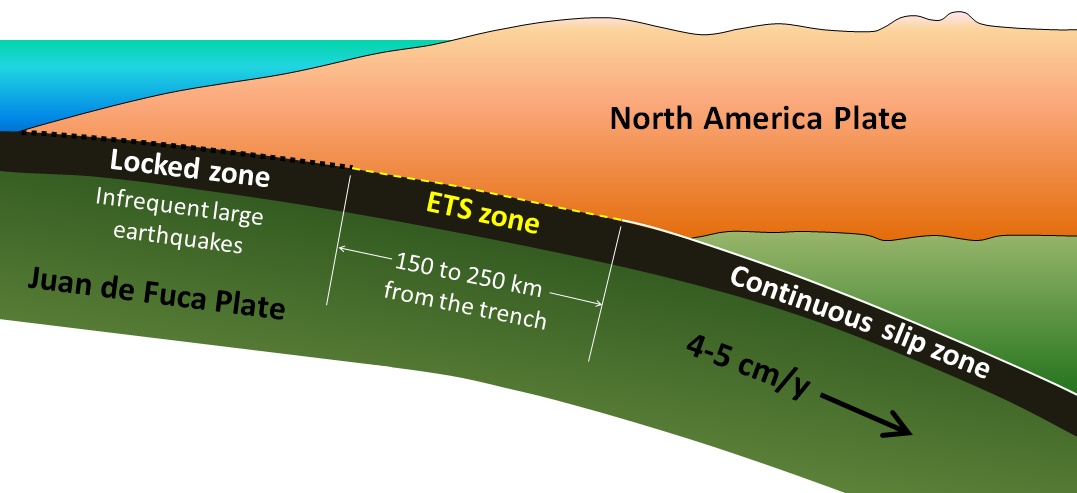
Episodic tremor and slip (ETS) is periodic slow sliding along part of a subduction boundary. It does not produce recognizable earthquakes, but does produce seismic tremor (observed as rapid seismic vibrations on instruments). It was first discovered on the Vancouver Island part of the Cascadia subduction zone by Geological Survey of Canada geologists Herb Dragert and Gary Rogers.20
The boundary between the subducting Juan de Fuca plate and the North America plate can be divided into three segments (Figure 12.7). The cold upper part of the boundary is the locked zone. There the plates are stuck together for long periods of time. When slip does occur, it generates very large earthquakes. The last time the locked zone along Canada’s west coast slipped was January 26, 1700. It caused an earthquake of magnitude 9. The warm lower part of the boundary, called the continuous slip zone, is sliding continuously because the warm rock is weaker. The central part of the boundary, the ETS zone, isn’t cold enough to be stuck, but isn’t warm enough to slide continuously. Instead it slips episodically approximately every 14 months for about 2 weeks, moving a few centimetres each time.
_](figures/12-earthquakes/figure-12-7.png)
Figure 12.7: Episodic tremor and slip along the Cascadia subduction zone. The Juan de Fuca plate is locked to the North American plate at the top of the subduction zone, but lower down it is slipping continuously. In the intermediate (ETS) zone, the plate alternately sticks and slips on a regular schedule. Source: Steven Earle (2015) CC BY 4.0 view source
It might seem that periodic slip along this part of the plate helps to reduce tension, and thus reduce the risk of a large earthquake. In fact, the opposite is likely the case. The movement along the ETS part of the plate boundary transfers stress to the adjacent locked part of the plate. During the two-week ETS period, the transfer of stress means an increased chance of a large earthquake.
Since 2003, ETS processes have also been observed in subduction zones in Mexico and Japan.
12.1.4.0.0.1 Additional Resources
IRIS Teachable Moment slides for the October 2012 Haida Gwaii earthquake
12.2 Measuring Earthquakes
The shaking from an earthquake travels away from the rupture in the form of seismic waves. Seismic waves are measured to determine the location of the earthquake, and to estimate the amount of energy released by the earthquake (its magnitude).
12.2.1 Types of Seismic Waves
Seismic waves are classified according to where they travel, and how they move particles.
12.2.1.1 Body Waves
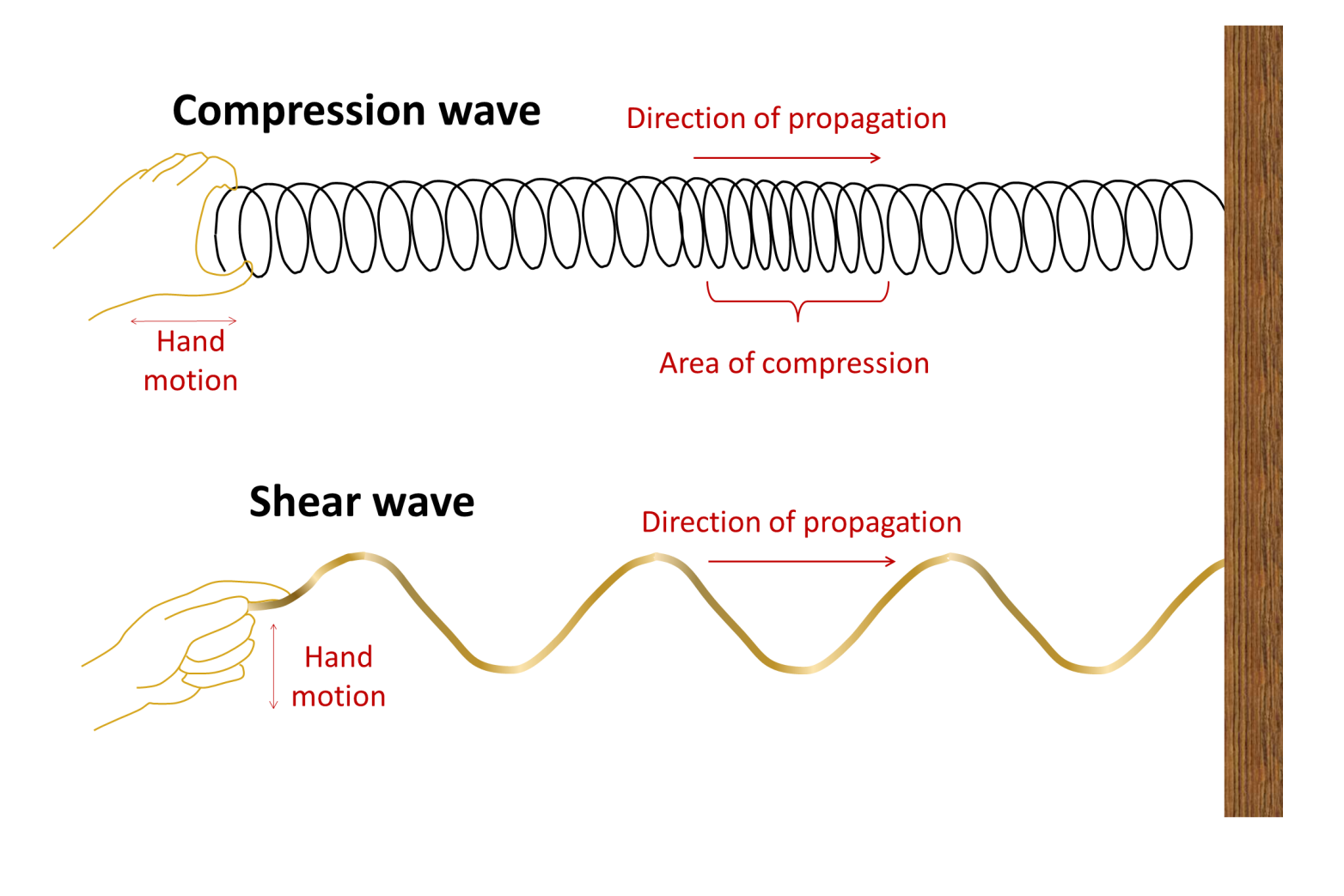
Seismic waves that travel through Earth’s interior are called body waves. P-waves are body waves that move by alternately compressing and stretching materials in the direction the wave moves. For this reason, P-waves are also called compression waves. The “P” in P-wave stands for primary, because P-waves are the fastest of the seismic waves. They are the first to be detected when an earthquake happens.
A P-wave can be simulated by fixing one end of a spring to a solid surface, then giving the other end a sharp push toward the surface (Figure 12.8, top). The compression will propagate (travel) along the length of the spring. Some parts of the spring will be stretched, and others compressed. Any one point on the spring will jiggle forward and backward as the compression travels along the spring.
._](figures/12-earthquakes/figure-12-8.png)
Figure 12.8: Seismic waves simulated using a spring and rope attached to a fixed surface. Top: P-waves travel as pulses of compression. Bottom: S-waves move particles at right angles to the direction of motion. Source: Karla Panchuk (2018) CC BY 4.0 modified after Steven Earle (2015) CC BY 4.0 view original.
S-waves are body waves that move with a shearing motion, shaking particles from side to side. S-waves can be simulated by fixing one end of a rope to a solid surface, then giving the other end a flick (Figure 12.8, bottom). Any one point on the rope will move from side to side at a right angle to the direction in which the snaking motion is traveling. The “S” in S-wave stands for secondary, because S-waves are slower than P-waves, and are detected after the P-waves are measured. S-waves cannot travel through liquids.
P-waves and S-waves can travel rapidly through geological materials, at speeds many times the speed of sound in air.
12.2.1.2 Surface Waves
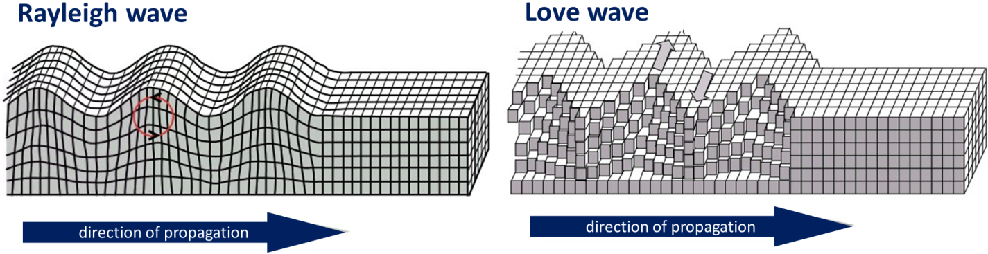
When body waves reach Earth’s surface, some of their energy is transformed into surface waves, which travel along Earth’s surface. Two types of surface waves are Rayleigh waves and Love waves (Figure 12.9). Rayleigh waves (R-waves) are characterized by vertical motion of the ground surface, like waves rolling on water. Love waves (L-waves) are characterized by side-to-side motion. Notice that the effects of both kinds of surface waves diminish with depth in Figure 12.9.
Surface waves are slower than body waves, and are detected after the body waves. Surface waves typically cause more ground motion than body waves, and therefore do more damage than body waves.
. Click the image for more attributions._](figures/12-earthquakes/figure-12-9.png)
Figure 12.9: Surface waves travel along Earth’s surface and have a diminished impact with depth. Rayleigh waves (left) cause a rolling motion, and Love waves (right) cause the ground to shift from side to side. Source: Steven Earle (2015) CC BY 4.0 view source. Click the image for more attributions.
12.2.2 Recording Seismic Waves Using a Seismograph
A seismometer is an instrument that detects seismic waves. An instrument that combines a seismometer with a device for recording the waves is called a s__eismograph__. The graphical output from a seismograph is called a seismogram. Figure 12.10 (right) shows how a seismograph works. The instrument consists of a frame or housing that is firmly anchored to the ground. A mass is suspended from the housing, and can move freely on a spring. When the ground shakes, the housing shakes with it, but the mass remains fixed. A pen attached to the mass moves up and down on a rotating drum of paper, drawing a wavy line, the seismogram. The seismograph in Figure 12.10 (right) is oriented to measure vertical ground motion. The photo on the left shows a seismograph oriented to record horizontal ground motion.
; Right: Karla Panchuk (2018) CC BY-SA 4.0, photo by Z22 (2014) CC BY-SA 3.0 [view source](https://commons.wikimedia.org/wiki/File:Seismogram_at_Weston_Observatory.JPG). Click the image for more attributions._](figures/12-earthquakes/figure-12-10.png)
Figure 12.10: How a seismograph records earthquakes. Source: Left- Karla Panchuk (2018) CC BY-NC-SA 4.0 modified after IRIS (2012) “How Does a Seismometer Work?” view source; Right: Karla Panchuk (2018) CC BY-SA 4.0, photo by Z22 (2014) CC BY-SA 3.0 view source. Click the image for more attributions.
The pen and drum of a mechanical seismograph record the motion of the ground relative to the mass. However, unless an earthquake causes a large amount of ground motion directly beneath the seismograph, the height of the wave recorded on paper might be very small, making the seismogram difficult to analyze. The seismograph on the right has a device to amplify the ground motion, drawing larger waves that are easier to study.
Modern seismographs record shaking as electrical signals, and are able to transmit those signals. This means seismologists need not return to the instrument to collect recordings before the records can be examined.
12.2.3 Finding The Location of an Earthquake
P-waves travel faster than S-waves. As the waves travel away from the location of an earthquake, the P-wave gets farther and father ahead of the S-wave. Therefore, the farther a seismograph is from the location of an earthquake, the longer the delay between when the P-wave arrival is recorded, and the S-wave arrival is recorded. The delay between the P-wave and S-wave arrival appears as a widening gap in a diagram of P-wave and S-wave travel times (Figure 12.11, grey lines).
P-wave and S-wave arrival times can be identified on seismograms. In the three seismograms in Figure 12.11, the arrivals of the P-waves and S-waves are marked with arrows, and the interval in minutes between the P-wave and S-wave arrivals are noted. The seismograms were recorded at three different seismic stations (earthquake monitoring locations equipped with seismographs). The distance of each station from the earthquake is determined by finding the distance along the graph where the gap between the P-wave and S-wave travel-time curves matches the delay between P-wave and S-wave arrivals on the seismogram.
_](figures/12-earthquakes/figure-12-11.png)
Figure 12.11: Using P-wave and S-wave travel times to determine how far seismic waves have travelled. Grey curves show the distance travelled by P-waves and S-waves after an earthquake occurs. P-waves are faster than S-waves, and the gap between them increases with time and distance. The delays between P-wave and S-wave arrivals on seismograms are matched to the curve to find the distances of seismic stations from the source of the seismic waves. Source: Karla Panchuk (2018) CC BY-NC-SA 4.0 modified after IRIS (n.d.) “How Are Earthquakes Located?” view source
The delay between the P-wave and S-wave arrival at a seismic station can indicate how far the station is from the source of the earthquake, but not the direction from which the seismic waves travelled. The possible locations of the earthquake can be represented on a map by drawing a circle around the seismic station, with the radius of the circle being the distance determined from the P-wave and S-wave travel times (Figure 12.12). If this is done for at least three seismic stations, the circles will intersect at the origin of the earthquake.
 Click the image for terms of use._](figures/12-earthquakes/figure-12-12.png)
Figure 12.12: Locating earthquakes by drawing three circles with radii of lengths determined from P-wave and S-wave travel times. Station names (SOCO, TEIG, SSPA) correspond to seismograms in Figure 12.11 Source: IRIS (n.d.) “How Are Earthquakes Located?” view source Click the image for terms of use.
12.2.4 How Big Was It?
Earthquakes can be described in terms of their magnitude, which reflects the amount of energy released by the shaking. They can also be described in terms of intensity, which characterizes the impact of the shaking on people and their surroundings.
12.2.4.1 Earthquake Magnitude
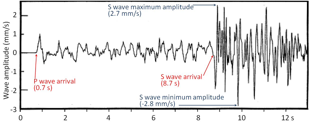
Earthquake magnitudes are determined by measuring the amplitudes of seismic waves. The amplitude is the height of the wave relative to the baseline (Figure 12.13). Wave amplitude depends on the amount of energy carried by the wave. The amplitudes of seismic waves reflect the amount of energy released by earthquakes.
_](figures/12-earthquakes/figure-12-13.png)
Figure 12.13: Seismogram for a small earthquake that occurred near Vancouver Island in 1997. The maximum amplitude of the S-wave is indicated. Source: Karla Panchuk (2018) CC BY 4.0 modified after Steven Earle (2015) CC BY 4.0 view source
The Richter magnitude scale uses the amplitudes of S-waves, and corrects for the decrease in amplitude that happens as the waves travel away from their source. The correction depends on how seismic waves interact with the specific rock types through which they travel, and therefore on local conditions, so the Richter magnitude is also referred to as the local magnitude.
While news reports about earthquakes might still refer to the “Richter scale” when describing magnitudes, the number they report is most likely the moment magnitude. The moment magnitude is calculated from the seismic moment of an earthquake. The seismic moment takes into account the surface area of the region that ruptured, how much displacement occurred, and the stiffness of the rocks. Moment magnitude can capture the difference between short earthquakes and longer ones resulting from larger ruptures, even of both types of earthquakes generate the same amplitude of waves. The moment magnitude scale is also better for earthquakes that are far from the seismic station. Seismic wave measurements are still used to determine the moment magnitude, however different waves are used than for the local magnitude scale.
The magnitude scale is a logarithmic one rather than a linear one- an increase of one unit of magnitude corresponds to a 32 times increase in energy release (Figure 12.14). There are far more low-magnitude earthquakes than high-magnitude earthquakes. In 2017 there were 7 earthquakes of M7 (magnitude 7) or greater, but millions of tiny earthquakes.
_](figures/12-earthquakes/figure-12-14.png)
Figure 12.14: Earthquake magnitude and corresponding energy release. Energy release increases by approximately 32 times for each unit change in magnitude. Source: IRIS (n.d.) “How Often Do Earthquakes Occur?” view source
12.2.4.2 Earthquake Intensity
Intensity scales were first used in the late 19th century, and then adapted in the early 20th century by Giuseppe Mercalli and modified later by others to form what we now call the Modified Mercalli Intensity Scale (Table 12.1). To determine the intensity of an earthquake, reports are collected about what people felt and how much damage was done. The reports are then used to assign intensity ratings to regions where the earthquake was felt. The Modified Mercalli Intensity Scale is as follows:
- I Not felt: Not felt except by a very few under especially favourable conditions
- II Weak: Felt only by a few persons at rest, especially on upper floors of buildings
- III Weak: Felt quite noticeably by persons indoors, especially on upper floors of buildings; many people do not recognize it as an earthquake; standing motor cars may rock slightly; vibrations similar to the passing of a truck; duration estimated
- IV Light: Felt indoors by many, outdoors by few during the day; at night, some awakened; dishes, windows, doors disturbed; walls make cracking sound; sensation like heavy truck striking building; standing motor cars rocked noticeably
- V Moderate: Felt by nearly everyone; many awakened; some dishes, windows broken; unstable objects overturned; pendulum clocks may stop
- VI Strong: Felt by all, many frightened; some heavy furniture moved; a few instances of fallen plaster; damage slight
- VII Very Strong: Damage negligible in buildings of good design and construction; slight to moderate in well-built ordinary structures; considerable damage in poorly built or badly designed structures; some chimneys broken
- VIII Severe: Damage slight in specially designed structures; considerable damage in ordinary substantial buildings with partial collapse; damage great in poorly built structures; fall of chimneys, factory stacks, columns, monuments, walls; heavy furniture overturned
- IX Violent
Damage considerable in specially designed structures; well-designed frame structures thrown out of plumb; damage great in substantial buildings, with partial collapse; buildings shifted off foundations - X Extreme: Some well-built wooden structures destroyed; most masonry and frame structures destroyed with foundations; rails bent
- XI Extreme: Few, if any (masonry), structures remain standing; bridges destroyed; broad fissures in ground; underground pipelines completely out of service; earth slumps and land slips in soft ground; rails bent greatly
- XII Extreme: Damage total; waves seen on ground surfaces; lines of sight and level distorted; objects thrown upward into the air
Intensity values are assigned to locations, rather than to the earthquake itself. This means that intensity can vary for a given earthquake, depending on the proximity to the epicentre and local conditions. For the 1946 M7.3 Vancouver Island earthquake, intensity was greatest in the central island region (Figure 12.15). In some communities within this region, chimneys were damaged on more than 75% of buildings. Some roads were made impassable, and a major rock slide occurred. The earthquake was felt as far north as Prince Rupert, as far south as Portland Oregon, and as far east as the Rockies, but with less intensity.
. Click the image for terms of use._](figures/12-earthquakes/figure-12-15.jpg)
Figure 12.15: Intensity map for the M7.3 Vancouver Island earthquake on June 23, 1946. Source: Earthquakes Canada, Natural Resources Canada (2016) view source. Click the image for terms of use.
Intensity estimates are important as a way to identify regions that are especially prone to strong shaking. A key factor is the nature of the underlying geological materials. The weaker the underlying materials, the more likely it is that there will be strong shaking. Areas underlain by strong solid bedrock tend to experience far less shaking than those underlain by unconsolidated river or lake sediments.
An example of this effect is the 1985 M8 earthquake that struck the Michoacán region of western Mexico, southwest of Mexico City. There was relatively little damage near the epicentre, but 350 km away in heavily populated Mexico City there was tremendous damage and approximately 5,000 deaths. The reason is that Mexico City was built largely on the unconsolidated and water-saturated sediment of former Lake Texcoco. These sediments resonate at a frequency of about two seconds, which was similar to the frequency of the body waves that reached the city. Consequently, the shaking was amplified. Survivors of the disaster recounted that the ground in some areas moved up and down by approximately 20 cm every two seconds for over two minutes. Damage was greatest to buildings between 5 and 15 storeys tall, because they also resonated at around two seconds, which amplified the shaking.
12.3 Earthquakes and Plate Tectonics
Bands of earthquakes trace out plate boundaries (coloured dots, Figure 12.16). The depths of earthquakes, and the width of the band, depend on the type of plate boundary. Mid-ocean ridges and transform margins have shallow earthquakes (usually less than 30 km deep), in narrow bands close to plate margins. Subduction zones have earthquakes at a range of depths, including some more than 700 km deep. Bands of earthquakes are wider along subduction zones because they take place throughout the subducting slab that extends beneath the opposing plate. Wide swaths of scattered earthquakes may correspond to continent-continent collision zones, such as between the Eurasian plate and the African, Arabian, and Indian plates to the south. Wide swaths of scattered earthquakes may also correspond to continental rift zones, such as in eastern Africa.
. Plate and ocean basin labels added. Click the image for terms of use._](figures/12-earthquakes/figure-12-16.png)
Figure 12.16: Earthquakes greater than magnitude 5, from 2000 to 2008. Bands of earthquakes mark tectonic plates. Narrow bands with shallow earthquakes (marked in red) indicate transform boundaries or mid-ocean ridge divergent boundaries. Wider bands with earthquakes at a range of depths are subduction zones. Wide bands of scattered earthquakes mark continent-continent convergent margins (e.g., between the Indian and Eurasian plates), or continental rift zones (e.g., in eastern Africa). Source: Lisa Christiansen, Caltech Tectonics Observatory (2008) view source. Plate and ocean basin labels added. Click the image for terms of use.
Earthquakes are also relatively common at a few locations away from plate boundaries. Some are related to the buildup of stress due to continental rifting or the transfer of stress from other regions, and some are not well understood. Locations include the Great Rift Valley area of Africa, the Lake Baikal area of Russia, and Tibet.
12.3.1 Earthquakes at Divergent and Transform Plate Boundaries
Earthquakes along divergent and transform plate margins are shallow (usually less than 30 km deep) because below those depths, rock is too hot and weak to avoid being permanently deformed by the stresses in those settings. If deformation is permanent, then removing the stress does not result in the rocks snapping back to their original shape. No snapping back means no shaking.
Mid-ocean ridge divergent plate margins are offset by numerous transform faults (Figure 12.17). The locations of earthquakes along mid-ocean ridges, and the mechanisms for causing them, depend on how rapidly the mid-ocean ridges are spreading. The Pacific-Antarctic Ridge (left) is spreading relatively rapidly at 42 to 94 mm/year, depending on the location along the ridge. Rapid spreading causes rocks near the axis of the spreading centre to be hot and weak. As a result, most of the earthquakes (white dots) are located along transform faults, where rocks are cooler and stronger. Along rapidly spreading ridges, new ocean crust is bent upward into wide, high ridges. As spreading proceeds and crust moves away from the ridge, the bend is relaxed, and the crust stretches and breaks. This triggers earthquakes many kilometres away from the ridge.
_](figures/12-earthquakes/figure-12-17.png)
Figure 12.17: Locations of earthquakes of magnitude 4 and greater from 1990 to 2010 along two mid-ocean ridges. Plate boundaries are marked in red. Arrows show the direction of plate motion. Left: Rapidly spreading Pacific-Antarctic ridge with earthquakes concentrated along transform faults. Right: Slowly spreading Southwest Indian Ridge, with earthquakes along both spreading segments and transform faults. Source: Karla Panchuk (2017) CC BY 4.0. Base maps with epicentres generated using the U. S. Geological Survey Latest Earthquakes website. Visit Latest Earthquakes
The Southwest Indian Ridge (right) spreads very slowly, at approximately 14 mm/year. Rocks are cooler and stronger along the slowly spreading ridge than along the rapidly spreading one. In the slow-spreading environment, earthquakes are generated when rocks along the ridge axis stretch and break. Earthquakes are more evenly distributed between divergent and transform segments of the boundary than they are along fast-spreading ridges.
Earthquakes in continental rift zones are also shallow, but scattered more broadly than those along mid-ocean ridges. Lake Baikal (Figure 12.28), the world’s oldest, deepest, and largest freshwater lake, formed 25 million years ago because of continental rifting. Note the scale in Figure 12.18, and compare how widely the earthquakes (blue dots) are spread in the Lake Baikal region, versus along the mid-ocean ridges in Figure 12.17.
_](figures/12-earthquakes/figure-12-18.png)
Figure 12.18: Blue circles mark the locations of earthquakes of M4 and greater from 1990 to 2010 along the Lake Baikal rift zone. White lines show some of the faults in the region. White lines with tick marks are normal faults related to spreading. Arrows show the direction of spreading. White lines without tick marks are transform faults. The Siberian Craton (shaded region) is strong 2 billion year old crust. Source: Karla Panchuk (2017) CC BY 4.0. Faults after U. S. Geological Survey (see references). Base maps (inset and rift views) with epicentres generated using the U. S. Geological Survey Latest Earthquakes website. Visit Latest Earthquakes
One reason for the difference in earthquake distribution in continental rift zones is that the rifts are only beginning to form. Faulting is “disorganized” within the continental crust. There is no well-established spreading centre, unlike mid-ocean ridges. Another reason is that the locations of faults, and thus earthquakes, in continental rift zones are affected by pre-existing geological structures within continental crust. In the case of the Lake Baikal rift, the strong, ancient crust of the Siberian Craton influences the orientation of the faults forming the rift. Faults run parallel to the craton near Lake Baikal. As rifting extends to the east, the part of the craton in the upper right of Figure 12.18 may deflect rifting southward.
12.3.2 Earthquakes at Convergent Boundaries
12.3.2.1 Subduction Zones
Along convergent plate margins with subduction zones, earthquakes range from shallow to depths of up to 700 km. Earthquakes occur where the two plates are in contact, as well as in zones of deformation on the overriding plate, and along the subducting slab deeper within the mantle. The result is that epicentres of earthquakes farther to the interior of the overriding plate will correspond to increasingly deep earthquakes.
Where the Pacific plate subducts beneath the North American plate, forming the Aleutian volcanic arc (Figure 12.19), earthquakes increase in depth moving northward, following the Pacific plate into the mantle. Earthquakes between 0 and 33 km deep (red circles) occur closest to the subduction zone (red line; teeth point in the direction of the subducting slab). While there is some overlap, earthquakes between 33 and 70 km deep (white circles) occur in a band that reaches farther the north. Farthest north are the epicentres for earthquakes between 70 and 300 km deep (green dots). The deepest earthquake during the seven year interval shown in Figure 12.19 is represented by the large green dot farthest to the north. It occurred at a depth of 265 km.
_](figures/12-earthquakes/figure-12-19.png)
Figure 12.19: Earthquakes of M4.5 and greater from 2010 to 2017 along the Aleutian Trench subduction zone (red line; teeth point in the direction of the subducting slab). White arrows show the directions of plate movement. Circle colours indicate the depths of earthquakes (see legend, lower left). Earthquakes become deeper moving north from the subduction zone. Source: Karla Panchuk (2017) CC BY 4.0. Base maps with epicentres generated using the U. S. Geological Survey Latest Earthquakes website. Visit Latest Earthquakes
Earthquakes occur in subduction zones for a variety of reasons. Stresses associated with the collision of two plates cause deformation in the overriding plate, and thus shallow earthquakes. Shallow earthquakes also happen on the subducting slab when a locked zone (orange line, Figure 12.20) ruptures. The locked zone is where the largest earthquakes on Earth, called megathrust earthquakes, occur. There is the potential for a wider rupture zone on a gently dipping subduction zone boundary compared to other boundaries.
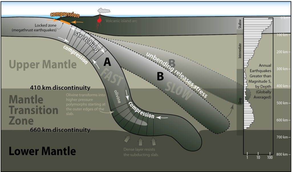
Figure 12.20: Factors contributing to earthquakes in subduction zones. Not all factors shown here are present in all subduction zones. Stress from bending, flexing, and stretching may cause ruptures. Changes in the mechanical properties of the mantle may affect how subucting slabs move, contributing additional stresses. The histogram at right shows the global average number of earthquakes at depth, for earthquakes greater than M5. The increase in earthquakes beneath 480 km may be caused in part by weakening as olivine transforms into high pressure/temperature polymorphs. Source: Karla Panchuk (2017) CC BY 4.0. Modified after Green et al. (2010).
If subduction is rapid, the subducting plate will bend more as it enters the mantle (slab A in Figure 12.20), causing the upper edge of the plate to stretch, and the interior and lower edge to be compressed. Stress from bending can cause shallow to intermediate earthquakes on these plates. Even without bending, the subducting slab can become stretched by its own weight as it falls into the mantle.
The 410 km and 660 km discontinuities in Figure 12.20 mark boundaries where minerals transform into other, denser minerals that are stable at higher pressures and temperatures. When the subducting slab reaches the 660 km discontinuity (the top of the lower mantle), the increase in density in the surrounding mantle may slow down the leading edge of the sinking slab. Earthquakes can be generated when the slab is compressed by the lower mantle resisting its motion at the same time that the upper part of the slab continues to fall.
Slower rates of subduction mean that the subducting slab will enter the mantle at a lower angle (slab B in Figure 12.20). These slabs might not have earthquakes from being bent downward into the mantle, as with slab A, but earthquakes may be triggered by changes in stress if the plate relaxes and unbends.
The bar chart on the right of Figure 12.20 shows global average number of earthquakes that occur at different depths. Earthquakes are most abundant at the surface, and then fall to a minimum at 300 km. The number of earthquakes remains low until almost 500 km depth, and reaches a second peak around 600 km depth. The second peak might be explained by interactions between the subducting plate and the dense mantle beneath the 660 km discontinuity, but another hypothesis is that it is related to delayed mineral transformations. The subducting slab warms as it goes deeper into the mantle, but the warming is not uniform. The outer edges of the slab will warm before the interior does. The 410 km discontinuity is where olivine is transformed into the minerals wadsleyite and ringwoodite under normal mantle pressure and temperature conditions. However, if the interior of the subducting slab is still too cool at that depth, olivine will be retained to depths below 410 km. Olivine weakens prior to transforming into the high pressure minerals, and the weakening may make it easier for the slab to rupture.
12.3.2.2 Continent-Continent Convergence Zones
Where continents collide, earthquakes are scattered over a much wider area compared to earthquakes along mid-ocean ridges, transform margins, or subduction zones. An example is where the Indian plate collides with the Eurasian plate (Figure 12.21). At one time, India was a separate continent, and ocean crust separated India from the Eurasian plate. For a time, a subduction zone existed where ocean lithosphere from the Indian plate subducted beneath the Eurasian plate. But when the two land masses finally met, they became locked together and the subduction zone was closed off. Today the Indian plate is still pushing against the Eurasian plate in the regions indicated by the red arrows in Figure 12.21. The collision is accommodated by transform boundaries along the Indian plate. Regions of overall transform motion are indicated in Figure 12.21 with blue arrows.
_](figures/12-earthquakes/figure-12-21.png)
Figure 12.21: Earthquakes of M4.5 and greater from 1990 to 2017 along the collision zone between the Indian and Eurasian plates. Red lines- plate boundaries; red arrows- collision zones; blue arrows- transform zones. Source: Karla Panchuk (2017) CC BY 4.0. Base maps with epicentres generated using the U. S. Geological Survey Latest Earthquakes website. Visit Latest Earthquakes
The majority of earthquakes in Figure 12.21 occur at depths less than 70 km, however they are still abundant down to 150 km, and extend to more than 300 km depth at some locations. Deeper earthquakes may be caused by continued northwestward subduction of part of the Indian plate beneath the Eurasian plate in this area. Even though the area is no longer a subduction zone, the subducted slab still remains, and is subject to stresses that can trigger earthquakes.
Some of the earthquakes in Figure 12.21 are related to the transform faults on either side of the Indian plate, and most of the others are related to the squeezing caused by the continued convergence of the Indian and Eurasian plates. That squeezing has caused the Eurasian plate to be thrust over the Indian plate, building the Himalayas and the Tibet Plateau to enormous heights. Most of the earthquakes of Figure 12.21 are related to the thrust faults shown in Figure 12.22 (and to hundreds of other similar ones that cannot be shown at this scale). The southernmost thrust fault in Figure 12.22 (the Main Boundary Fault) is equivalent to the convergent boundary in Figure 12.21.
 after D. Vuichard (Figure \@ref(fig:figure-2-3)) in Ives and Messerli (1989)._](figures/12-earthquakes/figure-12-22.png)
Figure 12.22: Schematic diagram of the India-Asia convergent boundary, showing examples of the types of faults along which earthquakes are focused. Source: Steven Earle (2015) CC BY 4.0 view source after D. Vuichard (Figure 2.3) in Ives and Messerli (1989).
12.3.3 Intraplate Earthquakes
Intraplate earthquakes (within-plate earthquakes) are those that occur away from plate boundaries. Some intraplate earthquakes are related to human activities. When humans trigger earthquakes it is referred to as induced seismicity. In Saskatchewan there have been 20 earthquakes since 1985 (all less than magnitude 4), and the majority occurred near potash mines. Excavation changes the stress in surrounding rocks, so earthquakes may occur in the rocks above excavated parts of the mine. In Alberta, induced seismicity is triggered by hydraulic fracturing operations when water pressure increases along existing faults, causing them to slip.
Intraplate earthquakes not related to human activities often occur along ancient rift zones. In eastern Canada, the Charlevoix seismic zone (approximately 100 km northeast of Québec City; Figure 12.23), is associated with a rift-zone faults that developed when an ancient ocean basin began to form more than 500 million years ago. Coincidentally, the rocks of the Charlevoix Seismic Zone are also fragmented because of a meteorite impact (the crater margin is indicated by the blue circle in Figure 12.23), weakening them further. While the Charlevoix zone is far from any boundary of the North American plate, tectonic forces acting on plate boundaries are still transmitted to the interior of the continent, contributing to the stress that causes the faults along the rift zone to rupture.
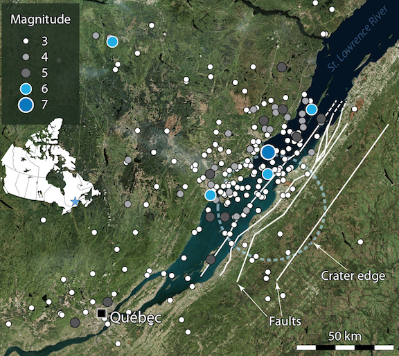
Figure 12.23: Charlevoix seismic zone, site of intraplate earthquakes. The location of the Charlevoix seismic zone is indicated by the star on the map of Canada. Dots indicate earthquake epicentres. The size of the dots indicates magnitude. White lines indicate fault segments. The dashed circle marks the edge of a crater formed by a meteorite impact 342 million years ago. Source: Karla Panchuk (2017) CC BY-SA 4.0. Epicentre data from Earthquakes Canada. Click the image for more attributions and data sources.
Intraplate earthquakes can be large earthquakes. The Charlevoix seismic zone has had five earthquakes of magnitudes between 6 and 7 since 1663. The New Madrid seismic zone in the Mississippi River Valley had a series of four earthquakes with magnitudes between 7 and 8 in the winter of 1811-1812. The population of the region was sparse at the time, but today there are major cities in the New Madrid seismic zone, including Memphis, Tennessee, and St. Louis, Missouri.
12.4 The Impacts of Earthquakes
Earthquakes can have direct impacts, such as structural damage to buildings from shaking, and secondary impacts, such as triggering landslides, fires, and tsunami. The types and extent of impacts will depend on local conditions where the earthquake strikes. The geological materials in the area matter, as does the type of terrain, and whether the region is near the coast or not. The extent of impact and type of damage will depend on whether the area is predominantly urban or rural, densely or sparsely populated, highly developed or underdeveloped. It will depend on whether the infrastructure has been designed to withstand shaking.
12.4.1 Damage to Structures from Shaking
As with the example of the 1985 Mexico earthquake, the geological foundations on which structures are built will affect the amount of shaking that occurs. Earthquakes produce seismic waves that vibrate at different rates, or frequencies. Waves with rapid vibrations have a high frequency, and waves with slower vibrations have lower frequencies.
The energy of the higher frequency waves tends to be absorbed by solid rock. Lower frequency waves pass through solid rock without being absorbed, but are absorbed and amplified by soft sediments. It is therefore very common to see much worse earthquake damage in areas underlain by soft sediments than in areas of solid rock. During the 1989 Loma Prieta earthquake, parts of a two-layer highway in the Oakland area near San Francisco collapsed where they were built on soft sediments (Figure 12.24).
_](figures/12-earthquakes/figure-12-24.jpg)
Figure 12.24: A collapsed section of the Cypress Freeway in Oakland California. Source: U. S. Geological Survey (1989) Public Domain view source
Building damage is also greatest in areas of soft sediments, and multi-storey buildings tend to be more seriously damaged than smaller ones. Buildings can be designed to withstand most earthquakes, and this practice is increasingly applied in earthquake-prone regions. Turkey is one such region, but even though Turkey had a relatively strong building code in the 1990s, adherence to the code was poor. Builders did whatever they could to save costs, including using inappropriate materials in concrete, and reducing the amount of steel reinforcing. The result was more than 17,000 deaths in the 1999 M7.6 Izmit earthquake (Figure 12.25). After two devastating earthquakes that year, Turkish authorities strengthened the building code further, but the new code has been applied only in a few regions, and enforcement of the code is still weak, as revealed by the amount of damage from a M7.1 earthquake in eastern Turkey in 2011.
; Right: USGS (1999) Public Domain [view source](https://commons.wikimedia.org/wiki/File:Izmit_eart3.jpg)_](figures/12-earthquakes/figure-12-25.png)
Figure 12.25: Damage from the 1999 M7.6 Izmit, Turkey earthquake. Source: Left; USGS (1999) Public Domain view source; Right: USGS (1999) Public Domain view source
Structures underlain by sediments may be at risk of another hazard, called liquefaction, in which sediment is transformed into a fluid. When water-saturated sediments are shaken, the grains may lose contact with each other, and no longer support one another. Water between the grains holds them apart, causing the sediment to turn to mud and flow. The loss of support can lead to the collapse of buildings or other structures that might otherwise have sustained little damage. During the 1964 M7.6 earthquake in Niigata, Japan, liquefaction caused buildings to sink into the sediments (Figure 12.26).
_](figures/12-earthquakes/figure-12-26.jpg)
Figure 12.26: Collapsed apartment buildings in the Niigata area of Japan. The material beneath the buildings was liquefied by the 1964 earthquake. Source: DOC/NOAA/NESDIS/NCEI (1964) Public Domain view source
Parts of the Fraser River delta are also prone to liquefaction-related damage. The region is characterized by a 2 m to 3 m thick layer of fluvial silt and clay above a layer of water-saturated fluvial sand that is at least 10 m thick (Figure 12.27). Under these conditions, seismic shaking can be amplified, and the sandy sediments will liquefy. This could lead to subsidence and tilting of buildings. Liquefaction can also contribute to slope failures and to fountains of sandy mud (sand volcanoes) in areas where there is loose saturated sand beneath a layer of more cohesive clay. Current building-code regulations in the Fraser delta area require that measures be taken to strengthen the ground beneath multi-story buildings prior to construction.
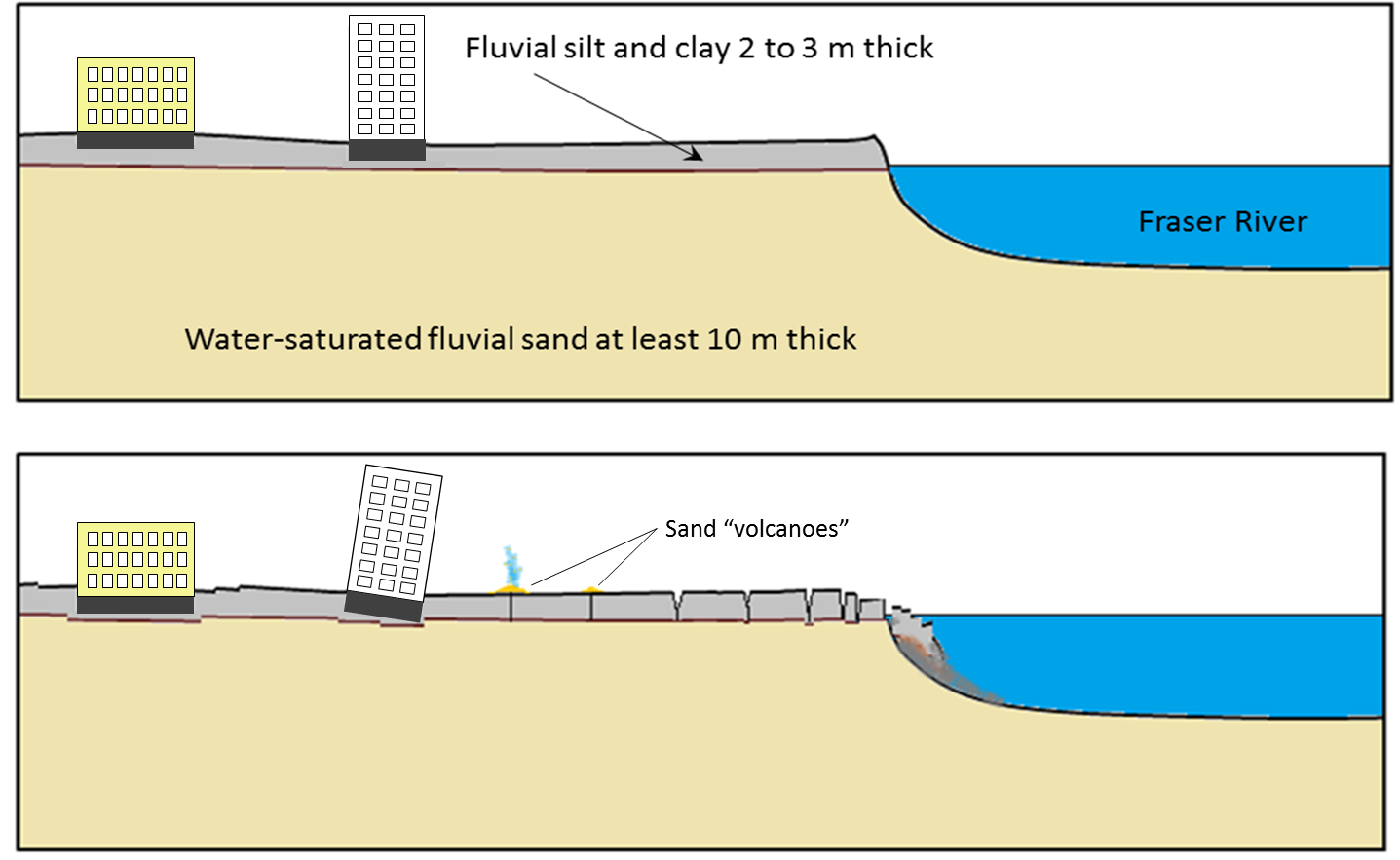](figures/12-earthquakes/figure-12-27.png)
Figure 12.27: Recent unconsolidated sedimentary layers in the Fraser River delta area (top) and the potential consequences in the event of a damaging earthquake. Source: Steven Earle (2015) CC BY 4.0 view source
12.4.1 Experiments with Liquefaction
To see liquefaction for yourself, go to a sandy beach and find a place near the water’s edge where the sand is wet. While standing in one place on a wet part of the beach, start moving your feet up and down at a frequency of about once per second. Within a few seconds the previously firm sand will start to lose strength, and you’ll gradually sink in up to your ankles.
If you can’t get to a beach, put some sand into a small container, saturate it with water, and then pour the excess water off. Shake the container gently to get the water to separate and then pour the excess water away. You may have to do this more than once. Place a small rock on the surface of the sand. It should sit there for hours without sinking in. Now, holding the container in one hand gently thump the side or the bottom with your other hand, about twice a second. The rock should gradually sink in as the sand around it becomes liquefied.
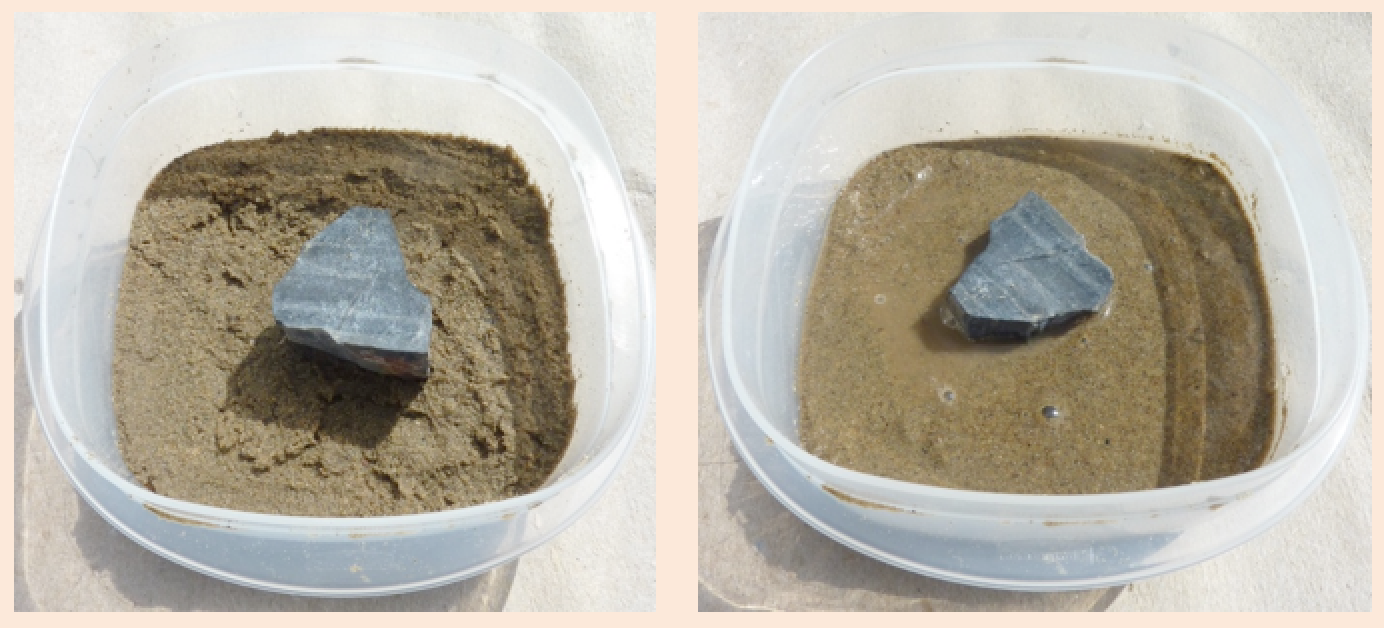_](figures/12-earthquakes/figure-12-28.png)
Figure 12.28: Fine, damp sand before shaking (left) and after (right). Source: Steven Earle (2015) CC BY 4.0 view source
As you were moving your feet up and down or thumping the container, it’s likely that you soon discovered the most effective rate for getting the sand to liquefy. Stepping up and down as fast as you can (several times per second) on the wet beach would not have been effective, nor would you have achieved much by stepping once every several seconds. The body of sand vibrates most readily in response to shaking that is close to its natural harmonic frequency, and liquefaction is also most likely to occur at that frequency.
12.4.2 Slope Failure
Ground shaking during an earthquake can be enough to weaken rock and loose materials to the point of failure. Earthquakes can also trigger failures on slopes that are already weak. In January of 2011 a M7.6 earthquake offshore of El Salvador triggered slope failures that killed nearly 600 people (Figure 12.29).
_](figures/12-earthquakes/figure-12-29.jpg)
Figure 12.29: A slope gives way in a suburb of San Salvador after the January 2001 earthquake offshore of El Salvador. This is one of hundreds of slope failures resulting from the earthquake. Source: U. S. Geological Survey (2001) Public Domain view source
12.4.3 Fires
Fires are commonly associated with earthquakes because gas lines rupture and electrical lines are damaged when the ground shakes. Most of the damage in the great 1906 San Francisco earthquake was caused by massive fires in the downtown area of the city (Figure 12.30). Some 25,000 buildings were destroyed by those fires, which were fueled by gas leaking from broken pipes. Fighting the fires was difficult because water mains had also ruptured. Today the risk of fires can be reduced through P-wave early warning systems if utility operators can decrease pipeline pressure and break electrical circuits.
_](figures/12-earthquakes/figure-12-30.jpg)
Figure 12.30: Fires in San Francisco following the 1906 earthquake. Source: Pillsbury Picture Co. (1906) Public Domain, courtesy of the Library of Congress Prints and Photographs Division view source
12.4.4 Tsunami
Large earthquakes that take place beneath the ocean have the potential to displace large volumes of water. In a subduction zone, for example, the overriding plate becomes distorted by elastic deformation. It is squeezed laterally and pushed up (Figure 12.31 top). When an earthquake happens, the plate rebounds over an area of thousands of square kilometres, generating waves- a tsunami (Figure 12.31, middle). The waves spread across the ocean at velocities of several hundred kilometres per hour. Tsunami can make it to the far side of an ocean in about the same time as a passenger jet.
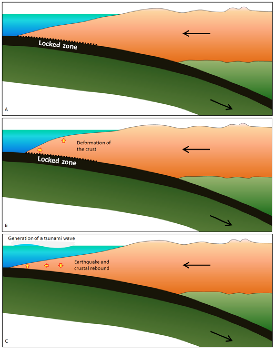. Bottom modified after COMET/UCAR (1997-2017) [view source](http://www.torbenespersen.dk/Publish/tsunami/media/graphics/comet_wave_transition.jpg). Click the image for COMET/UCAR attribution and terms of use._](figures/12-earthquakes/figure-12-31.png)
Figure 12.31: Tsunami triggered along a subduction zone. Top: The overriding crust is deformed because it is locked to the subducting slab. Middle: When the locked zone ruptures, the crust rebounds, and waves are created. Bottom: Tsunami waves have small amplitudes in the deep ocean, but once in shallow water, they slow down, causing the waves to become taller and closer together. Source: Karla Panchuk (2018) CC BY-NC-SA 4.0. Top and middle modified after Steven Earle (2015) CC BY 4.0 view source. Bottom modified after COMET/UCAR (1997-2017) view source. Click the image for COMET/UCAR attribution and terms of use.
Tsunami waves gain their height as they travel through shallower waters. In the deep ocean, the waves may be so small as to go undetected by ships, but when they are slowed down by interacting with the ocean floor, they can become much taller (Figure 12.31, bottom). In the tsunami following the 2004 Sumatra earthquake, the tallest waves were more than 30 m high.
Subduction earthquakes must be large to generate significant tsunami. Earthquakes with magnitude less than 7 do not typically generate significant tsunami because the amount of vertical displacement of the sea floor is minimal. Sea-floor transform earthquakes, even large ones (M7 to M8), don’t typically generate tsunami either, because the motion is mostly side to side, not vertical.
Tsunami can have an impact across an entire ocean basin. They spread across the ocean at velocities of several hundred kilometres per hour, and can make it to the far side of an ocean in about the same time as a passenger jet. In 1700 a rupture along the Cascadia thrust fault running from Vancouver Island to northern California resulted in a M9 earthquake. It generated a tsunami that travelled across the Pacific Ocean, and was recorded in Japan nine hours later. A computer simulation of the tsunami (Figure 12.32) shows how long it took tsunami waves from the Cascadia earthquake to travel across the Pacific Ocean, and how high the waves were. Notice that over all, the waves decrease in height moving away from the rupture, but they increase in height again as they reach the opposite side of the Pacific Ocean.
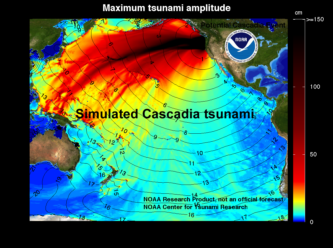 / [view context](https://nctr.pmel.noaa.gov/cascadia_simulated/index.html)_](figures/12-earthquakes/figure-12-32.png)
Figure 12.32: Computer simulation of the tsunami from the 1700 M9 Cascadia earthquake. Colours show open-ocean wave heights. Contours show travel time in hours. Tsunami wave heights increase as the tsunami reached the western margin of the Pacific ocean. Source: NOAA/PMEL/Center for Tsunami Research (2011) Public Domain view source / view context
12.5 Forecasting Earthquakes and Minimizing Impacts
It has long been a dream of seismologists, geologists, and public safety officials to be able to accurately predict the location, magnitude, and timing of earthquakes on time scales that would be useful for minimizing danger to the public and damage to infrastructure (e.g., weeks, days, hours). Many methods of prediction that have been explored. These include using observations of warning foreshocks, changes in magnetic fields, episodic tremor and slip, changing groundwater levels, strange animal behaviour, patterns in the timing between earthquakes, and how stress is transferred after a rupture. So far, none of these has provided a reliable method. Although there are some reports of successful earthquake predictions, they are rare, and many are surrounded by doubtful circumstances.
12.5.1 The Parkfield Prediction Experiment
There was great hope for earthquake predictions late in the 1980s when attention was focused on part of the San Andreas Fault at Parkfield, approximately 200 km south of San Francisco, California. Between 1881 and 1965 there were five earthquakes at Parkfield. They were spaced at approximately 20-year intervals, all confined to the same 20 km-long segment of the fault, and all very close to M6 (Figure 12.33). Both the 1934 and 1966 earthquakes were preceded by small foreshocks exactly 17 minutes before the main quake.
_](figures/12-earthquakes/figure-12-33.png)
Figure 12.33: Earthquakes on the Parkfield segment of the San Andreas Fault between 1881 and 2004. Source: Steven Earle (2015) CC BY 4.0 view source
The U. S. Geological Survey recognized this as an excellent opportunity to understand earthquakes and earthquake prediction, so they armed the Parkfield area with a huge array of geophysical instruments and waited. The next earthquake was expected to happen around 1987, but nothing happened! The “1987 Parkfield earthquake” finally struck in September 2004. Fortunately, all of the equipment was still there to record the earthquake, but it was no help from the perspective of earthquake prediction. There were no significant precursors to the 2004 Parkfield earthquake in any of the parameters measured, including tremors, changes in rock deformation, the magnetic field, the electrical conductivity of the rock, and creep (motion along the fault that is not accompanied by earthquakes). There was no foreshock. In other words, even though every available technique was used to monitor it, the 2004 earthquake came with no warning whatsoever.
12.5.2 Earthquake Probabilities
To be useful to the public and governments, earthquake predictions must be accurate _most _of the time, not just some of the time. If a prediction method is only accurate 10% of the time (and even that isn’t possible with the current state of knowledge), the public will lose faith in the process very quickly, and then will ignore all of the predictions. The hope for earthquake prediction is not dead, but it was hit hard by the Parkfield experiment.
Today the focus of efforts in earthquake-prone regions is to provide forecasts of earthquake probability. Earthquake probabilities express the likelihood that an earthquake of a given magnitude will occur at a location within a given period of time. An example of this approach for the San Francisco Bay region of California is shown in Figure 12.34. Based on a wide range of information, including past earthquake history, accumulated stress from plate movement, and known stress transfer, seismologists and geologists have predicted the likelihood of a M6.7 or greater earthquake on each of eight major faults that cut through the region. The greatest probabilities are on the San Andreas, Rogers Creek/Hayward faults, and Calaveras/Paicines faults. There is a 72% chance that a major and damaging earthquake will take place somewhere in the region prior to 2043.
_](figures/12-earthquakes/figure-12-34.png)
Figure 12.34: Earthquake outlook for 2014-2047. Probabilities for individual faults are marked on the faults. Source: U. S. Geological Survey (2014) Public Domain view report
12.5.3 Using Earthquake Probability Information
Decision makers can use forecasts of earthquake probability to assist with educating the public about earthquake risks, and to determine what action is necessary to make infrastructure earthquake-safe. Building safe infrastructure requires strong building codes, and enforcement of those codes. Building code compliance is robust in most developed countries, but is inadequate in many developing countries.
New buildings are not the only ones requiring attention. Existing buildings — especially schools and hospitals — and other structures such as bridges and dams, must also be made safe. British Columbia began a multi-billion-dollar program in 2004 to make public schools safer for students. The program is focused on older public schools, because, according to the government, those built since 1992 already comply with modern seismic codes. Some schools would require too much work to make upgrading economically feasible and they are replaced. Where upgrading is feasible, the school is assessed carefully before any upgrade work is initiated. The seismic mitigation program identified 346 schools as being at high risk and in need of upgrades. As of December 2017, upgrades were completed at 168 schools, 28 schools were under construction or had approval to proceed with construction, and 150 did not yet have plans in place for upgrades.
The program in British Columbia illustrates a challenge with seismic upgrades of public buildings, which is that governments must make adequate funds available for the upgrades to be done in a timely manner. The priority allocated to funding those projects will depend on how urgent the need for upgrades is considered to be, given other demands on public funds.
12.5.4 Earthquake Preparedness
Earthquake preparedness involves the formulation of public emergency plans, including escape routes, medical facilities, shelters, and food and water supplies. It also includes personal planning, such as emergency supplies (food, water, shelter, and warmth), escape routes from houses and offices, and communication strategies (with a focus on ones that don’t involve the cellular network).
12.6 Summary
The topics covered in this chapter can be summarized as follows:
12.6.1 What Is an Earthquake?
An earthquake is the shaking that results when a deformed body of rock snaps back to its original shape. The rupture is initiated at a point but quickly spreads across the area of a fault, with aftershocks initiated by stress transfer. Episodic tremor and slip is a periodic slow movement, accompanied by harmonic tremors, along the middle part of a subduction zone boundary.
12.6.2 Measuring Earthquakes
Earthquakes produce seismic waves that can be measured by a seismograph. The amplitudes of seismic waves are used to determine the amount of energy released by an earthquake- its magnitude. For the moment magnitude scale used today, the amount of energy released by an earthquake is proportional to the size of the rupture surface, the amount of displacement, and the strength of the rock. Intensity is a measure of the amount of shaking that occurs, and damage done at locations that experience an earthquake. Intensity will vary depending on the distance to the epicentre, the depth of the earthquake, and the type of geological materials present.
12.6.3 Earthquakes and Plate Tectonics
Most earthquakes happen at or near plate boundaries. Along divergent and transform boundaries earthquakes are shallow (less than 30 km depth), but at convergent boundaries they can be hundreds of kilometers beneath the surface. The largest earthquakes happen when a broad segment of the locked zone of a subduction zone ruptures. Intraplate earthquakes happen away from plate boundaries. They can be caused by human activities, or renewed motion on ancient faults.
12.6.4 The Impacts of Earthquakes
Damage to buildings is the most serious consequence of most large earthquakes. The amount of damage is related to the type and size of buildings, how they are constructed, and the nature of the material on which they are built. Other important consequences are fires, damage to bridges and highways, slope failures, liquefaction, and tsunami.
12.6.5 Forecasting Earthquakes and Minimizing Impacts
There is no reliable technology for predicting earthquakes, but the probability of one happening within a certain time period can be forecast. We can minimize earthquake impacts by ensuring that the public is aware of the risk, that building codes are enforced, that existing buildings like schools and hospitals are seismically sound, and that both public and personal emergency plans are in place.
12.7 Chapter Review Questions
What causes the shaking during an earthquake?
What is a rupture surface, and how does the area of a rupture surface relate to earthquake magnitude?
What is an aftershock and how are aftershocks related to stress transfer?
Episodic slip on the middle part of the Cascadia subduction zone is thought to increase the stress on the locked zone. Why?
What is the difference between the magnitude of an earthquake and its intensity?
How much more energy is released by a magnitude 7 earthquake compared to a magnitude 5 earthquake?
The images below show earthquake locations for three regions of ocean lithosphere. The colour scheme indicates the depths of earthquakes. a) The images show a subduction zone, a slowly spreading mid-ocean ridge, and a rapidly spreading mid-ocean ridge. Which is which? b) In the image with the subduction zone, which side is the subducting plate, and which is the overriding plate?
. Click the image for terms of use._](figures/12-earthquakes/figure-12-35.png)
Figure 12.35: Earthquakes along plate margins. Dots are colour coded according to depth. Source: Map details from Lisa Christiansen, Caltech Tectonics Observatory (2008) view source. Click the image for terms of use.
Why is earthquake damage likely to be more severe for buildings built on unconsolidated sediments as opposed to on solid rock?
Why are fires common during earthquakes?
What type of earthquake is likely to lead to a tsunami?
What did we learn about earthquake prediction from the 2004 Parkfield earthquake?
What are some of the things we should know about an area in order to help minimize the impacts of an earthquake?
What is the difference between earthquake prediction and forecasting earthquake probability?
12.8 Answers to Chapter Review Questions
Rocks under stress can deform elastically. When rocks break, or a rupture occurs along an existing fault, the deformed rocks snap back to their original shape, causing vibrations. The vibrations are the shaking felt during earthquakes.
The rupture surface is the surface over which there is displacement of rock during an earthquake. The magnitude of an earthquake is proportional to the area of the rupture surface.
An aftershock is an earthquake that is triggered when a rupture from a previous earthquake has transferred too much stress to rocks, causing further ruptures.
Episodic slip on the middle part of the Cascadia subduction zone decreases stress within that area, but some of that stress is transferred to the locked zone along the plate boundary. This increases the amount of stress on the locked part.
Magnitude is the amount of energy released by an earthquake. Each earthquake has only one magnitude, although there are different ways of measuring it, and they may give slightly different results. Intensity is a measure of the amount of damage done or what people felt. Intensity varies depending on the distance to the epicentre and the type of rock or sediment underlying an area.
Each unit increase in magnitude corresponds to a 32x increase in energy. The difference between M5 and M7 is two units of magnitude. An earthquake that is two magnitude units larger would release 32 x 32 = 1,024 times as much energy.
- A: Slowly spreading mid-ocean ridge- earthquakes are shallow and evenly distributed; B: Subduction zone- earthquakes range in depth; C: Rapidly-spreading mid-ocean ridge- earthquakes are shallow, and occur in patches, corresponding to a greater likelihood of earthquakes where transform faults offset ridges.
- The plate to the right of the chain of earthquakes is the subducting plate. The earthquakes increase in depth moving from right to left, indicating that the subducting slab is getting deeper farther to the left.
Unconsolidated sediments, especially if they are saturated with water, can lose strength when subjected to earthquake shaking. This can cause buildings to subside or tilt. Unconsolidated sediments can also amplify the vibrations of an earthquake.
Gas lines and electrical transmission wires are typically damaged during an earthquake, and this can lead to serious fires.
A large subduction-zone earthquake (greater than M7.5) can generate a tsunami because those earthquakes result in sufficient vertical displacement of the sea floor.
The 2004 Parkfield earthquake showed that we cannot rely on foreshocks to predict earthquakes, or on any of the many other parameters that were being carefully measured around Parkfield in the years leading up to the quake.
We should know about the history of past large earthquakes, the typical locations of small earthquakes, the types of geological materials beneath the surface (especially soft water-saturated sediments), the types of infrastructure that is present, and the various ways that people can be evacuated from an area or assistance can be brought in.
Forecasting involves estimating the risk of an earthquake happening in a region within a period of time. Prediction involves stating that an earthquake is likely to happen at a certain location on a specific day or month or year in the future. With our current state of knowledge of earthquakes, prediction is not possible.
12.9 References
Milne, W. G. (1955). Seismology in British Columbia. The Journal of the Royal Astronomical Society of Canada XLIX(4), 141 - 150. Read the paper
Ministry for Culture and Heritage (2017). Christchurch earthquake kills 185. Visit website
Wang, K., Jiangheng, H., Schulzeck, F., Hyndman, R. D., and Riedel, M. (2015). Thermal Condition of the 27 October 2012 Mw 7.8 Haida Gwaii Subduction Earthquake at the Obliquely Convergent Queen Charlotte Margin. Bulletin of the Seismological Society of America, 105(2B), 1290–1300. doi: 10.1785/0120140183
Ammon, C. J. (2001). Earthquake Size Visit website
12.9.0.0.0.1 References
Bao, X., and Eaton, D. W. (2016). Fault activation by hydraulic fracturing in western Canada. Science 354(6318), 1406-1409. doi: 10.1126/science.aag2583
Buck, W. R., Lavier, L. L., & Poliakov, A. N. B. (2005). Modes of faulting at mid-ocean ridges. Nature 434(7034), 719-23. doi: 10.1038/nature03358
Coastal and Marine Geology Program, U. S. Geological Survey (n.d.). Lake Baikal - A Touchstone for Global Change and Rift Studies. Visit website
DeMets, C., Gordon, R. G., & Argus, D. F. (2010). Geologically current plate motions. Geophysical Journal International 181, 1-80. doi: 10.1111/j.1365-246X.2009.04491.x
Earthquakes Canada, Natural Resources Canada (2016) Earthquake zones in Eastern Canada Visit website
Gendzwill, D. J., Horner, R. B., & Hasegawa, H. S. (1982). Induced earthquakes at a potash mine near Saskatoon, Canada. Canadian Journal of Earth Science 19, 466-475. doi: 10.1139/e82-038
Green, H. W. II, Chen, W.-P., & Brudzinski, M. R. (2010). Seismic evidence of negligible water carried below 400-km depth in subducting lithosphere. Nature 467, 828-830. doi:10.1038/nature09401
Hongyu, Y., Liu, Y., Harrington, R. M., & Lamontagne, M. (2016). Seismicity along St. Lawrence Paleorift Faults Overprinted by a Meteorite Impact Structure in Charlevoix, Québec, Eastern Canada. Bulletin of the Seismological Society of America 106(6), 2663-2673. doi: https://doi.org/10.1785/0120160036
Ives, J. D., Messerli, B. (1989). The Himalayan Dilemma: Reconciling development and conservation. New York: Routledge. Access this book courtesy of the New Zealand Digital Library, University of Waikato
Myhill, R., & Warren, L. M. (2012). Fault plane orientations of deep earthquakes in the Izu-Bonin-Marianas subduction zone. _Journal of Geophysical Research 117, _B06307. doi:10.1029/2011JB009047
Nishikawa, T., & Ide, S. (2015). Background seismicity rate at subduction zones linked to slab-bending-related hydration. _Geophysical Research Letters 42, _7081-7089. doi: 10.1002/2015GL064578
Sloan, R. A., Jackson, J. A., McKenzie, D., & Priestley, K. (2011). Earthquake depth distributions in central Asia, and their relations with lithosphere thickness, shortening and extension. Geophysics Journal International 185, 1-29. doi: 10.1111/j.1365-246X.2010.04882.x
Earthquakes Canada, Natural Resources Canada (2016). The M9 Cascadia Megathrust Earthquake of January 26, 1700. Visit website
University Corporation for Atmospheric Research (2010). Propagation. Tsunamis. Visit website
U. S. Geological Survey (1989). The Severity of an Earthquake. USGS General Interest Publication 1989-288-913 view source
U. S. Geological Survey (2014). Indian Ocean Tsunami Remembered — Scientists reflect on the 2004 Indian Ocean that killed thousands. Visit website
Finn, W. D. L., & Dexter, A. (2012). Risk Management Plan for School Seismic Mitigation Program. View report
Province of British Columbia (n.d.). Seismic Mitigation Program. Visit website
Province of British Columbia (2017). Seismic Mitigation Program Progress Report. View report
Rogers, G. and Dragert, H. (2003). Episodic tremor and slip on the Cascadia subduction zone: The chatter of silent slip. Science, 300, 1942-1943.↩︎
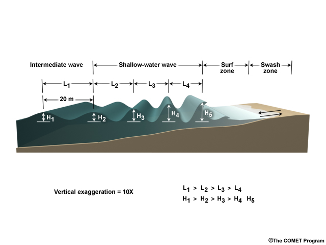