Chapter 19 Measuring Geological Time
Adapted from Physical Geology, First University of Saskatchewan Edition (Tim Prokopiuk and Karla Panchuk) and Physical Geology (Steven Earle)
](figures/19-measuring-geological-time/figure-19-1.jpg)
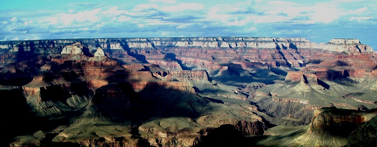
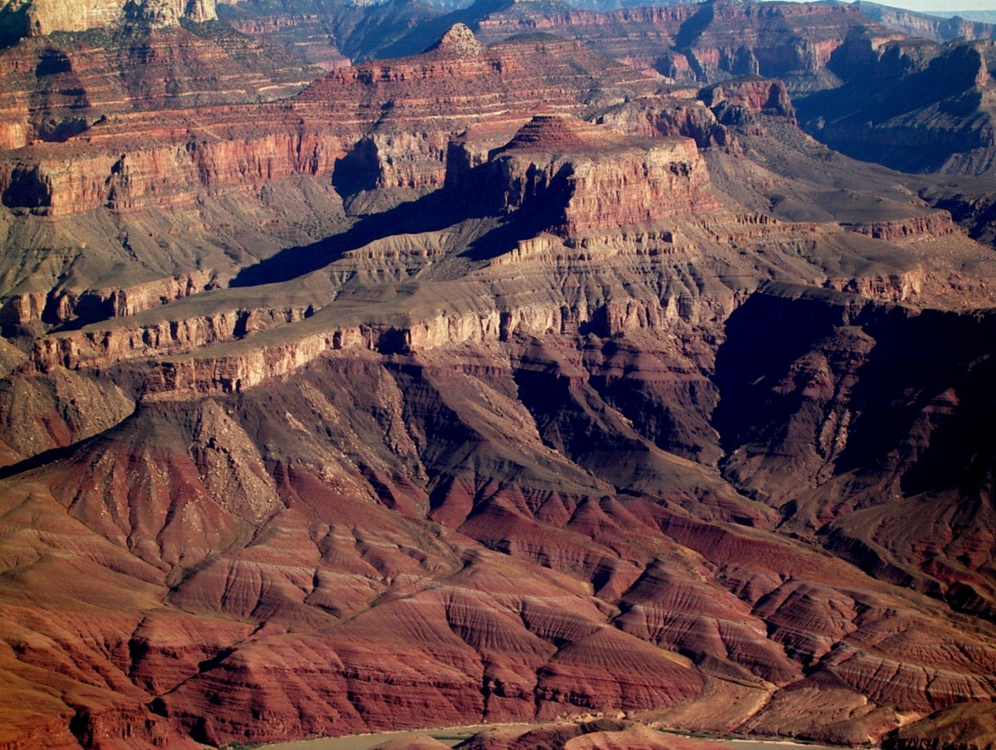
Figure 19.1: Arizona’s Grand Canyon is an icon for geological time; 1,450 million years are represented by this photo. The light-coloured layers of rocks at the top formed at ~ 250 Ma, and the dark ones at the bottom of the canyon at ~ 1,700 Ma. Source: Steven Earle (2015) CC BY 4.0 view source
Learning Objectives
After reading this chapter and answering the review questions at the end, you should be able to:
- Apply basic geological principles to determine the relative ages of rocks.
- Explain the difference between relative and absolute age-dating techniques.
- Summarize the history of the geological time scale and the relationships between eons, eras, periods, and epochs.
- Understand the importance and significance of unconformities.
- Estimate the age of a rock based on the fossils that it contains.
- Use isotopic data to estimate the absolute age of a rock.
- Describe some applications and limitations of isotopic techniques for absolute geological dating.
- Describe the techniques for dating geological materials using tree rings and magnetic data.
- Explain why an understanding of geological time is critical to both geologists and the public in general.
Time is the dimension that sets geology apart from most other sciences. Geological time is vast, and Earth has changed tremendously during this time. Even though most geological processes are very, very slow, the vast amount of time that has passed has allowed for the formation of extraordinary geological features, as shown in Figure 19.1
We have numerous ways of measuring geological time. We can tell the relative ages of rocks (e.g., whether one rock is older than another) based on their spatial relationships, we can use fossils to date sedimentary rocks because we have a detailed record of the evolution of life on Earth, and we can use a range of isotopic techniques to determine the absolute ages (in millions of years) of igneous and metamorphic rocks.
But just because we can measure geological time doesn’t mean that we understand it. One of the biggest hurdles faced by geology students—and geologists as well—in understanding geology is to really come to grips with the slow rates at which geological processes happen, and the vast amount of time involved.
19.1 The Geological Timescale
James Hutton (1726-1797) was a Scottish geologist, considered by some to be the father of modern Geology. Hutton studied present-day processes and applied his observations to the rock record in order to understand what he saw there. Such a method is now encapsulated in the principle of uniformitarianism, which states that the present is the key to the past. Given that many geological processes that we can see happening around us occur at very slow rates, Hutton concluded that geological time must be very long indeed to account for the large changes apparent in the rock record. But this principle needs to be taken with a grain of salt: there are some processes that have occurred in the past that are no longer occurring (e.g., eruption of ultramafic lavas), as well as some processes that occur so irregularly that we have not yet witnessed such an event in historic time (e.g., impact of a large asteroid with Earth).
William Smith worked as a surveyor in the coal-mining and canal-building industries in south-western England in the late 1700s and early 1800s. While doing his work, he had many opportunities to observe Paleozoic and Mesozoic sedimentary rocks of the region, and he did so in a way that few had done before. Smith noticed the textural similarities and differences between rocks in different locations. More importantly, he discovered that fossils could be used to correlate rocks of the same age. Smith is credited with formulating the principle of faunal succession, the concept that specific types of organisms lived during different time intervals. He used the principle of faunal succession to great effect in his monumental project to create a geological map of England and Wales, published in 1815.
Inset into Smith’s great geological map is a small diagram showing a schematic geological cross-section extending from the Thames estuary of eastern England to the west coast of Wales. Smith showed the sequence of rocks, from the Paleozoic rocks of Wales and western England, through the Mesozoic rocks of central England, to the Cenozoic rocks of the area around London (Figure 19.2).
._](figures/19-measuring-geological-time/figure-19-2.png)
Figure 19.2: William Smith’s “Sketch of the succession of strata and their relative altitudes,” an inset on his geological map of England and Wales (with era names added). Source: Steven Earle (2015) CC BY 4.0 view source, modified after William Smith (1815) Public Domain view map.
Smith did not put any dates on these rocks, because he didn’t know them. But he was aware of the principle of superposition, the idea developed much earlier by the Danish theologian and scientist Nicholas Steno, that young sedimentary rocks form on top of older ones. Therefore, Smith knew that this diagram represented a stratigraphic column. And since almost every period of the Phanerozoic is represented along this section through Wales and England, it is also a primitive geological time scale.
Smith’s work set the stage for the naming and ordering of the geological time periods, which was initiated around 1820, first by British geologists, and later by other European geologists. Many of the periods are named for places where rocks of that age are found in Europe, such as Cambrian for Cambria in Wales, Devonian for Devon in England, Jurassic for the Jura Mountains in France and Switzerland, and Permian for the Perm region of Russia. Some are named for the type of rock that is common during that age, such as Carboniferous for the coal-bearing rocks of England, and Cretaceous for the chalks of England and France.
The early time scales were only relative because 19th century geologists did not know the absolute ages of rocks. This information was not available until the development of isotopic dating techniques early in the 20th century.
The geological timescale is currently maintained by the International Commission on Stratigraphy (ICS), which is part of the International Union of Geological Sciences. The time scale is continuously being updated as we learn more about the timing and nature of past geological events. View the ICS timescale.
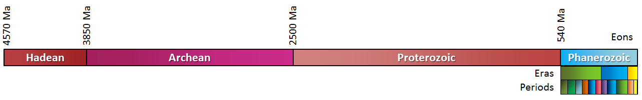
Geological time has been divided into four eons: Hadean, Archean, Proterozoic, and Phanerozoic (Figure 19.3). The first three of these eons represent almost 90% of Earth’s history. Rocks from the Phanerozoic (meaning “visible life”) are the most commonly exposed rocks on Earth, and they contain evidence of life forms with which we are familiar.
_](figures/19-measuring-geological-time/figure-19-3.png)
Figure 19.3: The eons of Earth’s history. Source: Karla Panchuk (2018) CC BY 4.0, modified after Steven Earle (2015) CC BY 4.0 view source
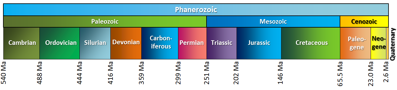
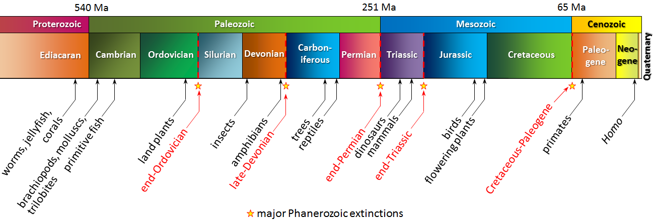
The Phanerozoic — the past 541 Ma of Earth’s history — is divided into three eras: the Paleozoic (“early life”), the Mesozoic (“middle life”), and the Cenozoic (“new life”), and each era is divided into periods (Figure 19.4). Most of the organisms with which we share Earth evolved into familiar forms at various times during the Phanerozoic.
_](figures/19-measuring-geological-time/figure-19-4.png)
Figure 19.4: The eras (middle row) and periods (bottom row) of the Phanerozoic. Source: Karla Panchuk (2018) CC BY 4.0, modified after Steven Earle (2015) CC BY 4.0 view source
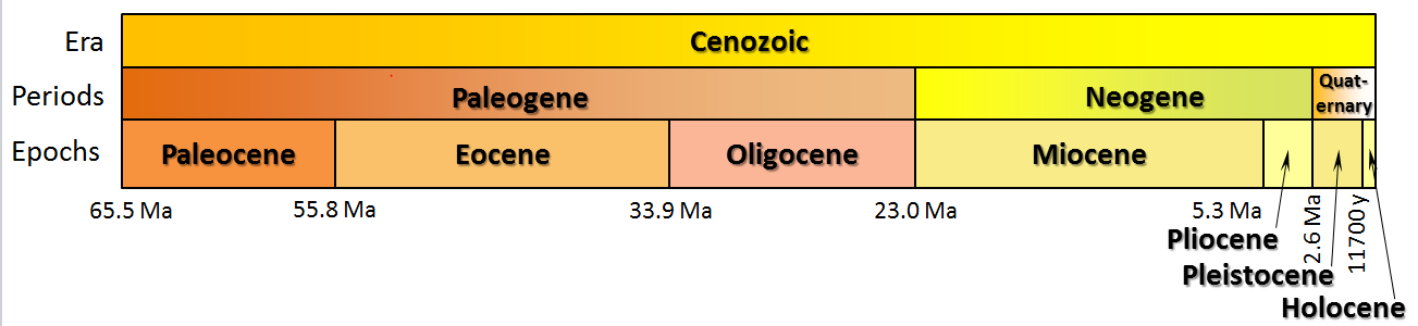
The Cenozoic, representing the past 66 Ma, is divided into three periods, the Paleogene, Neogene, and Quaternary; and seven epochs (Figure 19.5). Non-avian dinosaurs became extinct at the start of the Cenozoic, after which birds and mammals radiated to fill the available habitats. Earth was very warm during the early Eocene, and has cooled steadily ever since. Glaciers first appeared on Antarctica in the Oligocene and then on Greenland in the Miocene. By the Pleistocene, glaciers covered much of North America and Europe. The most recent of the Pleistocene glaciations ended ~11,700 years ago. The current epoch is known as the Holocene. Epochs are further divided into ages.
_](figures/19-measuring-geological-time/figure-19-5.png)
Figure 19.5: The periods and epochs of the Cenozoic Era. Source: Karla Panchuk (2018) CC BY 4.0, modified after Steven Earle (2015) CC BY 4.0 view source
Most of the boundaries between the periods and epochs of the geological timescale have been fixed on the basis of significant changes in the fossil record. For example, the boundary between the Cretaceous and the Paleogene coincides exactly with the extinction of the dinosaurs. This is not a coincidence. Many other types of organisms went extinct at this time, and the boundary between the two periods marks the division between sedimentary rocks containing Cretaceous organisms below, and those containing Paleogene organisms above.
19.2 Relative Dating Methods
19.2.1 Relative Dating Principles
The simplest and most intuitive way of dating geological features is to look at the relationships between them. There are a few simple rules for doing this. But caution must be taken, as there may be situations in which the rules are not valid, so local factors must be understood before an interpretation can be made. These situations are generally rare, but they should not be forgotten when unraveling the geological history of an area.
The principle of superposition states that sedimentary layers are deposited in sequence, and the layers at the bottom are older than those at the top. This situation may not be true, though, if the sequence of rocks has been flipped completely over by tectonic processes, or disrupted by faulting.
The principle of original horizontality indicates that sediments are originally deposited as horizontal to nearly horizontal sheets. At a broad scale this is true, but at a smaller scale it may not be. For example, cross-bedding forms at an appreciable angle, where sand is deposited upon the lee face of a ripple. The same holds true of delta foreset beds (Figure 19.6).
_](figures/19-measuring-geological-time/figure-19-6.png)
Figure 19.6: A cross-section through a river delta forming in a lake. The delta foresets are labeled “Delta deposits” in this figure, and you can quickly see that the front face of the foresets are definitely not deposited horizontally. Source: AntanO (2017) CC BY 4.0 view source
The principle of lateral continuity states that sediments are deposited such that they extend laterally for some distance before thinning and pinching out at the edge of the depositional basin. But sediments can also terminate against faults or erosional features (see unconformities below), so may be cut off by local factors.
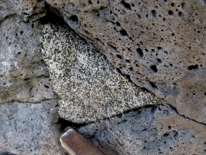
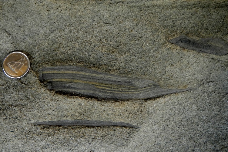
The principle of inclusions states that any rock fragments that are included in a rock must be older than the rock in which they are included. For example, a xenolith in an igneous rock, or a clast in sedimentary rock must be older than the rock that includes it (Figure 19.7). A possible situation that would violate this principle is the following: an igneous dyke may intrude through a sequence of rocks, hence is younger than these rocks (see the principle of cross-cutting relationships below). Later deformation may cause the dyke to be pulled apart into small pieces, surrounded by the host rocks. This situation can make the pieces of the dyke appear to be xenoliths, but they are younger than the surrounding rock in this case.
/ [right](http://opentextbc.ca/geology/wp-content/uploads/sites/110/2015/07/sandstone.jpg)_](figures/19-measuring-geological-time/figure-19-7.png)
Figure 19.7: Applications of the principle of inclusion. Left- A xenolith of diorite incorporated into a basalt lava flow, Mauna Kea volcano, Hawai’i. The lava flow took place some time after the diorite crystallized (hammer head for scale). Right- Rip-up clasts of shale embedded in Gabriola Formation sandstone, Gabriola Island, BC. The pieces of shale were eroded as the sand was deposited, so the shale is older than the sandstone. Source: Karla Panchuk (2018) CC BY 4.0. Photographs by Steven Earle (2015) CC BY 4.0 view sources left/ right
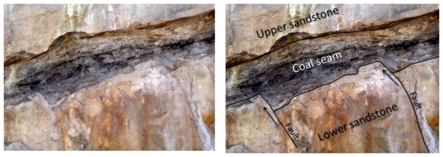
The principle of cross-cutting relationships states that any geological feature that cuts across or disrupts another feature must be younger than the feature that is disrupted. An example of this is given in Figure 19.8, which shows three different sedimentary layers. The lower sandstone layer is disrupted by two faults, so we can infer that the faults are younger than this layer. But the faults do not appear to continue into the coal seam, and they certainly do not continue into the upper sandstone. So we can infer that coal seam is younger than the faults (because the coal seam cuts across them). The upper sandstone is youngest of all, because it lies on top of the coal seam. An example that violates this principle can be seen with a type of fault called a growth fault. A growth fault is a fault that continues to move as sediments are continuously delivered to the hangingwall block. In this case, the lower portion of the fault that cuts the lower sediments may have originally formed before the uppermost sediments were deposited, despite the fault cutting through all of the sediments, and appearing to be entirely younger than all of the sediments.
_](figures/19-measuring-geological-time/figure-19-8.png)
Figure 19.8: Superposition and cross-cutting relationships in Cretaceous Nanaimo Group rocks in Nanaimo BC. The coal seam is about 50 cm thick. Source: Steven Earle (2015) CC BY 4.0 view source
The principle of baked contacts states that the heat of an intrusion will bake (metamorphose) the rocks in close proximity to the intrusion. Hence the presence of a baked contact indicates the intrusion is younger than the rocks around it. If an intrusive igneous rock is exposed via erosion, then later buried by sediments, the surrounding rocks will not be baked, as the intrusion was already cold at the time of sediment deposition. But baked contacts may be difficult to discern, or may be minimally developed to absent when the intrusive rocks are low in volume or felsic (relatively cool) in composition.
The__ principle of chilled margins__ states that the portion of an intrusion that has cooled and crystallized next to cold surrounding rock will form smaller crystals than the portion of the intrusion that cooled more slowly deeper in the instrusion, which will form larger crystals. Smaller crystals generally appear darker in colour than larger crystals, so a chilled margin appears as a darkening of the intrusive rock towards the surrounding rock. This principle can be used to distinguish between an igneous sill, which will have a chilled margin at top and bottom, and a subaerial lava flow, which will have a chilled margin only at the bottom.
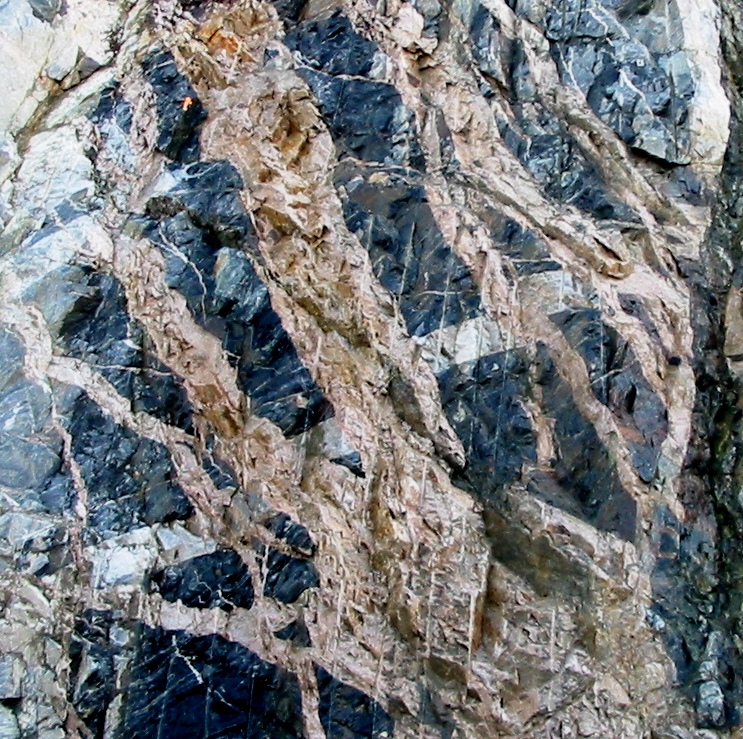
Exercise: Cross-Cutting Relationships
The outcrop in Figure 19.9 has three main rock types:
- Buff/pink felsic intrusive igneous rock present as somewhat irregular masses trending from lower right to upper left
- Dark grey metamorphosed basalt
- A 50 cm wide light-grey felsic intrusive igneous dyke extending from the lower left to the upper right – offset in several places Using the principle of cross-cutting relationships outlined above, determine the relative ages of these three rock types.
Note: The near-vertical stripes are blasting drill holes. The image is about 7 m across.
_](figures/19-measuring-geological-time/figure-19-9.jpg)
Figure 19.9: Outcrop from Horseshoe Bay, BC. Source: Steven Earle CC BY 4.0 view source
19.2.2 Unconformities
An unconformity represents an interruption in the process of deposition of sediments. Recognizing unconformities is important for understanding time relationships in sedimentary sequences. An unconformity is visible in the Grand Canyon (Figure 19.10, white dashed line) above Proterozoic rocks that were tilted and then eroded to a flat surface prior to deposition of the younger Paleozoic rocks. The difference in time between the youngest of the Proterozoic rocks and the oldest of the Paleozoic rocks is nearly 300 million years. Tilting and erosion of the older rocks took place during this time, and if there were any deposition occurring in this area during this time, erosion removed those sediments.
_](figures/19-measuring-geological-time/figure-19-10.png)
Figure 19.10: Angular unconformity in the Grand Canyon in Arizona, with a sketch of rock orientations. The tilted rocks at the bottom are part of the Proterozoic Grand Canyon Group (aged 825 to 1,250 Ma). The flat-lying rocks at the top are Paleozoic (540 to 250 Ma). The boundary between the two (dashed white line) represents a time gap of nearly 300 million years. Source: Karla Panchuk (2018) CC BY 4.0. Photograph by Steven Earle (2015) CC BY 4.0 view source
There are four types of unconformities, reflecting different arrangements and types of rocks above and below the surface of non-deposition or erosion (Table 19.1, Figure 19.12).
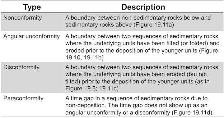
Figure 19.11: Types of Unconformities. Source: Karla Panchuk (2018) CC BY 4.0, modified after Steven Earle (2015) CC BY 4.0. Click the image for a text version of this table.
_](figures/19-measuring-geological-time/figure-19-11.png)
Figure 19.12: The four types of unconformities: (a) a nonconformity between non-sedimentary rock and sedimentary rock, (b) an angular unconformity, (c) a disconformity between layers of sedimentary rock, where the older rock has been eroded but not tilted, and (d) a paraconformity where there is a long period (millions of years) of non-deposition between two parallel layers. Source: Steven Earle (2015) CC BY 4.0 view source
Exercise: Relative Dating with Unconformities
- The surfaces G and H in Figure 19.13 are unconformities. What kind?
- If erosion at the surface stopped and sediments were deposited once again, what kind of unconformity would exist between the layer I and younger rocks?
- Provide a list of the events that affected the rocks in Figure 19.13 in order from the oldest event to the most recent event. Note that C and D are faults. The sedimentary rocks labelled A are folded, but the other sedimentary rocks are horizontal.
 _](figures/19-measuring-geological-time/figure-19-12.png)
Figure 19.13: Block diagram showing sedimentary and igneous rocks affected by faults, folds, and erosion. Source: Karla Panchuk (2018) CC BY-SA 4.0, modified after Woudloper (2009) CC BY-SA 1.0 view source
19.3 Dating Rocks Using Fossils
Geologists obtain a wide range of information from fossils. They help us to understand evolution, and life in general; they provide critical information for understanding depositional environments and changes in Earth’s climate; and they can be used to date rocks.
Although the recognition of fossils goes back hundreds of years, the systematic cataloguing and assignment of relative ages to different organisms from the distant past—paleontology—only dates back to the earliest part of the 19th century. The oldest undisputed fossils are from rocks dated ~3.5 Ga, and although fossils this old are typically poorly preserved and are not useful for dating rocks, they can still provide important information about conditions at the time. The oldest well-understood fossils are from rocks dating back to ~600 Ma, and the sedimentary record from this time forward is rich in fossil remains that provide a detailed record of the history of life. However, as anyone who has gone hunting for fossils knows, this does not mean that all sedimentary rocks have visible fossils or that they are easy to find. Fossils alone cannot provide us with numerical ages of rocks, but over the past century geologists have acquired enough isotopic dates from rocks associated with fossiliferous rocks (such as igneous dykes cutting through sedimentary layers) to be able to put specific time limits on most fossils.
A selective history of life on Earth over the past 600 million years is provided in Figure 19.14 The major groups of organisms that we are familiar with appeared between the late Proterozoic and the Cambrian (~600 Ma to ~541 Ma). Plants, which originally evolved in the oceans as green algae, invaded land during the Ordovician (~450 Ma). Insects, which evolved from marine arthropods, invaded land during the Devonian (400 Ma), and amphibians (i.e., vertebrates) invaded land about 50 million years later. By the late Carboniferous, trees had evolved from earlier plants, and reptiles had evolved from amphibians. By the mid-Triassic, dinosaurs and mammals had evolved from reptiles and reptile ancestors, Birds evolved from dinosaurs during the Jurassic. Flowering plants evolved in the late Jurassic or early Cretaceous. The earliest primates evolved from other mammals in the early Paleogene, and the genus _Homo _evolved during the late Neogene (~2.8 Ma).
_](figures/19-measuring-geological-time/figure-19-13.png)
Figure 19.14: A selective summary of life on Earth during the late Proterozoic and the Phanerozoic. The top row shows geological eras, and the lower row shows geological periods. Source: Steven Earle (2015) CC BY 4.0 view source
If we understand the sequence of evolution on Earth, we can apply this knowledge to determining the relative ages of rocks. This is William Smith’s principle of faunal succession, although in spite of the name, it can apply to fossils of plants and simple organisms as well as to fauna (animals).
The Phanerozoic Eon has witnessed five major extinctions (stars in Figure 19.14). The most significant of these was at the end of the Permian, which saw the extinction of over 80% of all species, and over 90% of all marine species. Most well-known types of organisms that survived were still severely impacted by this event. The second most significant extinction occurred at the Cretaceous-Paleogene boundary (K-Pg, also known the Cretaceous-Tertiary or K-T extinction). At that time, ~75% of marine species disappeared, as well as dinosaurs (but not birds) and pterosaurs. Other species were badly reduced but survived, and then flourished in the Paleogene. The K-Pg extinction may have been caused by the impact of a large asteroid (10 km to 15 km in diameter) and/or volcanic eruptions associated with the formation of the Deccan Traps, but it is generally agreed that the other four Phanerozoic mass extinctions had other causes, although their exact nature is not clearly understood.
It is not a coincidence that the major extinctions all coincide with boundaries of geological periods and/or eras. Paleontologists have placed most of the divisions of the geological time scale at points in the fossil record where there are major changes in the type of fossils observed.
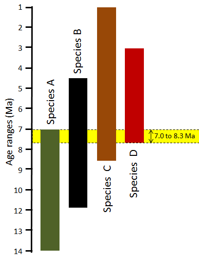
If we can identify a fossil, and we know when the organism lived, we can assign a range of time to the formation of the sediments in which the organism was preserved when it died. This range might be several millions of years, because some organisms survived for a very long time. If the rock we are studying has several types of fossils in it, and we can assign time ranges to all of these fossils, we may be able to narrow the time range for the age of the rock considerably (Figure 19.15).
_](figures/19-measuring-geological-time/figure-19-14.png)
Figure 19.15: Application of bracketing to constrain the age of a rock based on the presence of several fossils. The yellow bar represents the time range during which each of the four species (A – D) existed on Earth. Although each species lived for several millions of years, we can narrow down the age of the rock to a span of just 1.3 Ma during which all four species coexisted. Source: Steven Earle (2015) CC BY 4.0 view source
Some organisms survived for a very long time, and are not particularly useful for dating rocks. Sharks, for example, have existed for over 400 million years, and the great white shark has survived for 16 million years so far. Organisms that lived for relatively short time periods are particularly useful for dating rocks, especially if they were distributed over a wide geographic area and hence can be used to compare rocks from different regions. These are known as index fossils. There is no specific limit on how short the time span has to be for a fossil to qualify as an index fossil. Some such organisms lived for millions of years, and others for much less than a million years.
Some well-studied groups of organisms qualify as __biozone __fossils because, although the genera and families lived over a long time, each species lived for a relatively short time and can be easily distinguished from others on the basis of specific features. For example, ammonites have a distinctive feature known as the suture line, where the internal shell layers that separate the individual chambers (septae) meet the outer shell wall (Figure 19.16). These suture lines are sufficiently variable to identify species that can be used to estimate the relative or absolute ages of the rocks in which they are found.
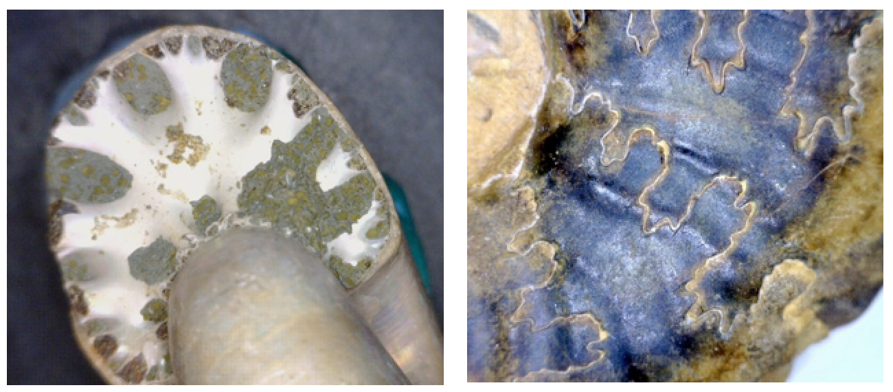_](figures/19-measuring-geological-time/figure-19-15.png)
Figure 19.16: The septum of an ammonite (white part, left), and the suture lines where the septae meet the outer shell (right). Source: Steven Earle (2015) CC BY 4.0 view source
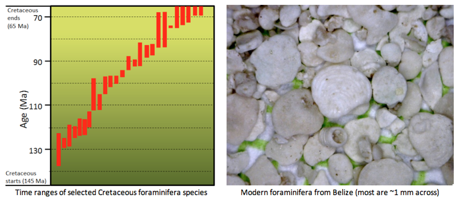
Foraminifera—small, calcium carbonate-shelled marine organisms that originated during the Triassic and are still alive today—are also useful biozone fossils. Numerous different foraminifera lived during the Cretaceous Period, some for over 10 million years, but others for less than 1 million years (Figure 19.17). If the foraminifera in a rock can be identified to the species level, the rock’s age can be determined.
](figures/19-measuring-geological-time/figure-19-16.png)
Figure 19.17: Time ranges for Cretaceous foraminifera (left), and modern foraminifera from the Ambergris area of Belize (right)._ Source: Left- Steven Earle (2015) CC BY 4.0, from data in Scott (2014). Right- Steven Earle (2015) CC BY 4.0 _view source
Exercise: Dating Rocks Using Index Fossils
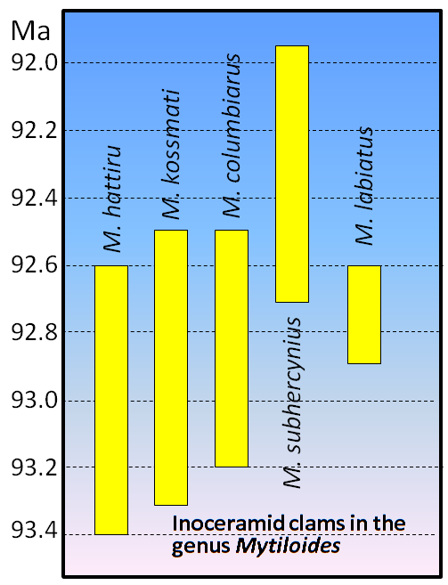
Figure 19.18 shows the age ranges for some late Cretaceous inoceramid clams in the genus Mytiloides. Using the bracketing method described above, determine the possible age range of a rock in which all five of these organisms were found.
How would the age range change if M. subhercynius were not present in the rock?
_](figures/19-measuring-geological-time/figure-19-17.png)
Figure 19.18: Inoceramid ranges. Source: Steven Earle (2015) CC BY 4.0, from data in Harries et al. (1996). View source
19.3.1 Correlation
Geologists employ relative age dating techniques to correlate rocks between regions. Correlation seeks to relate the geological history between regions, by relating the rocks in one region to those in another.
There are different techniques of correlation. The easiest technique is to correlate by rock type, or lithology, called lithostratigraphic correlation. In this method, specific rock types are related between regions. If a sequence of rocks at one site consists of a sandstone unit overlain by a limestone unit, then a unit of shale, and the exact same sequence of rocks—sandstone, limestone, shale—occurs at a nearby site, lithostratigraphic correlation means assuming that the rocks at both sites are in the same rocks. If you could see all of the rock exposed between the two sites, the units would connect with one another. The problem with this type of correlation is that some rocks may only have formed locally, or may pinch out between the two sites, and therefore not be present at the site to which a correlation is being attempted.
Another technique, biostratigraphic correlation, involves correlation based on fossil content. This technique uses fossil assemblages (fossils of different organisms that occur together) to correlate rocks between regions. The best fossils to use are those that are widely spread, abundant, and lived for a relatively short period of time.
Yet another technique, chronostratigraphic correlation, is to correlate rocks that have the same age. This can be the most difficult way to correlate, because rocks are generally diachronous. That is, if we trace a given rock unit across any appreciable lateral distance, the age of that rock actually changes. To give a familiar example, when you go to the beach, you know that the beach itself and the lake bottom in the shallow water is sandy. But if you swim out to deeper water and touch bottom, the bottom feels muddy. The difference in sediment type has to do with the energy of deposition, with the waves at and near the beach keeping any fine sediments away, only depositing them in deeper quieter waters. If you think of this example in time, you realize that the sand at and near the beach is being deposited at the same time as the mud in deeper water. But if lake levels drop, the beach sands will slowly migrate outwards and cover some of the deeper water muds. If lake levels rise, the deeper water muds will slowly migrate landwards and cover some of the shallower water sands. This is an example of Walther’s Law, which states that sedimentary rocks that we see one on top of each other in the rock record actually formed adjacent to one another at the time of deposition. In order to correlate rock units in time, we must target marker beds that formed instantaneously. An example of such would be an ash layer from a nearby volcano that erupted and blanketed an entire region in ash. But such marker beds are usually rare to absent, making such correlation extremely difficult.
19.4 Isotopic Dating Methods
19.4.1 Isotope Pairs
Originally, fossils only provided us with relative ages because, although early paleontologists understood biological succession, they did not know the absolute ages of the different organisms. It was only in the early part of the 20th century, when isotopic dating methods were first applied, that it became possible to discover the absolute ages of the rocks containing fossils. In most cases, we cannot use isotopic techniques to directly date fossils or the sedimentary rocks in which they are found, but we can constrain their ages by dating igneous rocks that cut across sedimentary rocks, or volcanic ash layers that lie within sedimentary layers.
Isotopic dating of rocks, or the minerals within them, is based upon the fact that we know the decay rates of certain unstable isotopes of elements, and that these decay rates have been constant throughout geological time. It is also based on the premise that when the atoms of an element decay within a mineral or a rock, they remain trapped in the mineral or rock, and do not escape.
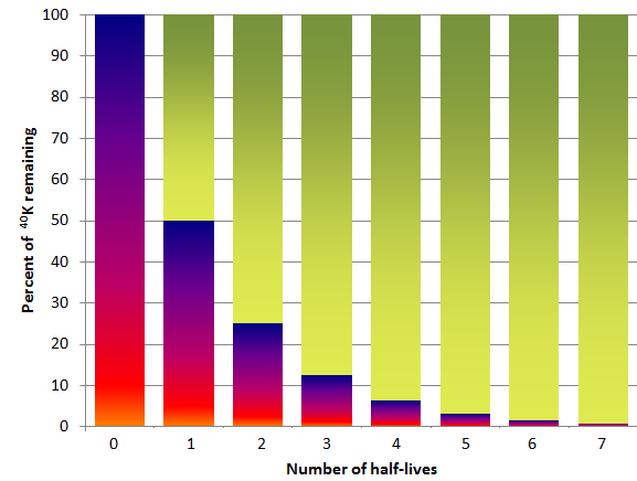
One of the isotope pairs commonly used to date rocks is the decay of 40K to 40Ar (potassium-40 to argon-40). 40K is a radioactive isotope of potassium that is present in very small amounts in all minerals that contain potassium. It has a half-life of 1.3 billion years, meaning that over a period of 1.3 Ga one-half of the 40K atoms in a mineral or rock will decay to 40Ar, and over the next 1.3 Ga one-half of the remaining atoms will decay, and so forth (Figure 19.19). 40K is called the parent isotope, and 40Ar the daughter isotope, as the parent gives way to the daughter during radioactive decay.
_](figures/19-measuring-geological-time/figure-19-18.png)
Figure 19.19: The decay of 40K over time. Each half-life is 1.3 billion years, so after 3.9 billion years (three half-lives) 12.5% of the original 40K will remain. The red-blue bars represent 40K and the green-yellow bars represent 40Ar. Source: Steven Earle (2015) CC BY 4.0 view source
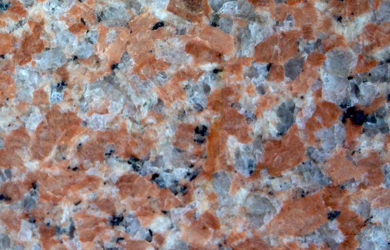
In order to use the K-Ar dating technique, we need to have an igneous or metamorphic rock that includes a potassium-bearing mineral. One good example is granite, which contains the mineral potassium feldspar (Figure 19.20). Potassium feldspar does not contain any argon when it forms. Over time, the 40K in the feldspar decays to 40Ar. The atoms of 40Ar remain embedded within the crystal, unless the rock is subjected to high temperatures after it forms. The sample must be analyzed using a very sensitive mass-spectrometer, which can detect the differences between the masses of atoms, and can therefore distinguish between 40K and the much more abundant 39K. The minerals biotite and hornblende are also commonly used for K-Ar dating.
_](figures/19-measuring-geological-time/figure-19-19.jpg)
Figure 19.20: Crystals of potassium feldspar (pink) in a granitic rock are candidates for isotopic dating using the K-Ar method because they contained potassium and no argon when they formed. Source: Steven Earle (2015) CC BY 4.0 view source
There are many isotope pairs that can be employed in dating igneous and metamorphic rocks (see Table 19.2), each with its strengths and weaknesses. In the above example, the daughter isotope 40Ar is naturally a gas, and can escape the potassium feldspar quite easily if the feldspar is exposed to heating during metamorphism, or interaction with hydrothermal fluids. Hence we must closely examine the feldspar mineral to determine if there is any evidence of alteration. If some 40Ar has been lost, but the sample is dated anyway, an age that is too young will be calculated.
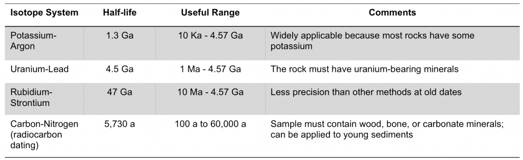
Figure 19.21: Commonly used isotope systems for dating geological materials. Source: Steven Earle (2015) CC BY 4.0. Click the table for a text version.
Each parent isotope has a certain half-life, which ranges from microseconds to billions of years, depending upon the isotope. In dating rocks, we need to select an isotope pair with a parent isotope that has a reasonable half-life. This means that the half-life must not be too short or too long. If the half-life is too short, then most of the parent isotope will have decayed to form the daughter isotope. If we cannot measure the amount of parent isotope very accurately, which will be impossible to do if there is only the tiniest amount of parent isotope left, our calculated age will have huge errors associated with it. The same applies if the half-life is too long. In this case, very little of the daughter isotope will have formed, and our inability to measure the small amount of daughter isotope accurately will again result in huge errors in our calculated age.
Another complicating factor is whether the mineral of interest incorporated any of the daughter isotope into its structure at the time of formation. When we select a mineral and an isotope pair to date that mineral, we make the assumption that all of the daughter isotope we find in the mineral was produced in the mineral by radioactive decay of the parent isotope. But if the mineral formed with some daughter isotope already present in its structure, then the age we calculate will be too old.
A more robust mineral to use to date certain types of igneous and metamorphic rocks is zircon. Zircon is a mineral that incorporates uranium into its structure at the time of formation. One of the isotopes of uranium decays to lead with a long half-life (see Table 19.2). Zircon is a mineral of choice for dating because it takes no lead into its structure when it forms, so any lead present is due entirely to the radioactive decay of the uranium parent. Another reason is because zircon is a very resistant mineral. It can handle exposure to hydrothermal fluids, and all but the highest grades of metamorphism, and not lose any of the parent or daughter isotopes. Hence the age that we calculate tends to be very accurate. One drawback is that zircon tends to form only in felsic igneous rocks. Hence if we are trying to date a mafic igneous rock, we must choose a different mineral.
19.4.2 The Meaning of a Radiometric Date
When we employ isotopic methods on minerals we are measuring an age date. Generally, an age date refers to the time since a mineral crystallized from molten rock (magma or lava). This is when the elements that make up the mineral get locked into the mineral’s structure. But as we have already seen, elevated temperatures can cause elements to escape from a mineral, without the mineral melting. Hence when we date a mineral, we may be dating the time since the mineral crystallized from a melt, or the time since the mineral last experienced a period of heating above its Curie point, which is the temperature beyond which the mineral is able to lose (or gain) elements from its structure, without melting. So we have to know something about the rock before we forge ahead to measure an age. We may choose a mineral and isotope pair that are very resistant to metamorphism, so that we can “see through” the metamorphism, and determine the original age that the mineral crystallized from a melt. Or we may be interested in the age of the metamorphic event itself, so choose a mineral and isotope pair that is susceptible to resetting the isotopic clock during metamorphism (such as by losing all of the daughter isotope).
Absolute age dating is a powerful tool for unraveling the geological history of a region, but we have seen that we must ultimately rely upon igneous rocks (that may have later metamorphosed) for the minerals that we are able to date (see the next section for issues with dating sedimentary rocks directly). Another issue with absolute age dating is that it is expensive, with a single analysis costing several hundreds of dollars. Hence geologists never forget their relative age dating principles, and are always applying them in the field to determine the sequence of events that formed the rocks in a region.
Exercise: Combining Absolute Ages with Relative Dating
The age dates for three igneous rock layers are given. Use relative dating techniques to determine the age ranges for the sets of sedimentary units A, B, and C.
_](figures/19-measuring-geological-time/figure-19-20.png)
Figure 19.22: A sequence of igneous and sedimentary layers. Age dates are given for the igneous layers. Source: Karla Panchuk (2018) CC BY-SA 4.0, modified after Jill Curie (2014) CC BY-SA 3.0 view source
19.4.3 Isotope Dating Techniques and Sedimentary Rocks
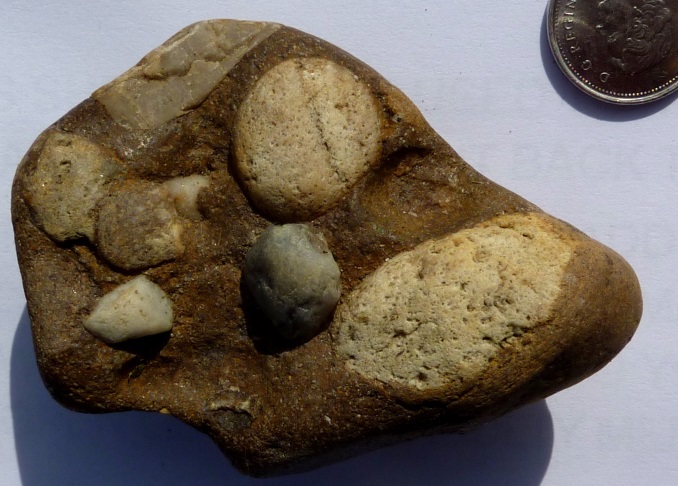
A clastic sedimentary rock (e.g., conglomerate, Figure 19.23) is made up of older rock and mineral fragments. These fragments were derived from weathering and erosion of pre-existing rocks. The process of forming a sedimentary rock from sediments generally occurs at low temperatures, so the minerals are not heated beyond their Curie points. Hence the minerals still preserve their original ages (either igneous crystallization age, or a metamorphic age).
_](figures/19-measuring-geological-time/figure-19-21.jpg)
Figure 19.23: Conglomerate is a sedimentary rock consisting of large rounded clasts surrounded by finer-grained material. Source: Steven Earle (2015) CC BY 4.0 view source
In almost all cases, the fragments have come from a range of source rocks that all formed at different times. If we dated a number of individual grains in the sedimentary rock, we would likely get a range of different dates, all older than the age of the sedimentary rock. The most that such ages gleaned from a sedimentary rock can tell us is a maximum age of the sedimentary rock. It might be possible to date some chemical sedimentary rocks isotopically, but there are no useful isotopes that can be used on old chemical sedimentary rocks.
19.4.4 Radiocarbon Dating
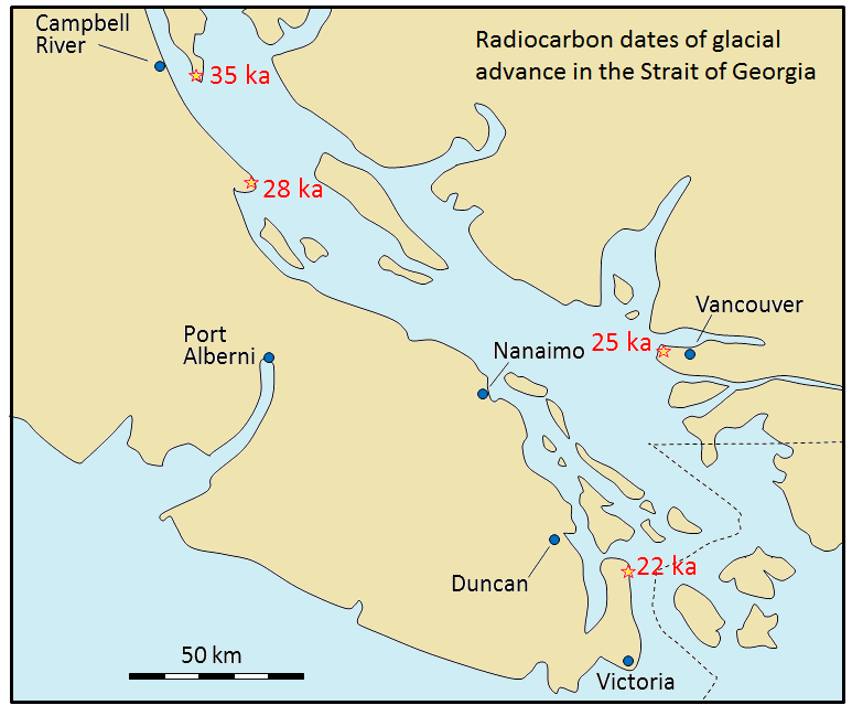
Radiocarbon dating (using 14C) can be applied to many geological materials, including sediment and sedimentary rocks, but only if the materials in question are younger than ~60 ka, and contain organic material. Beyond this time, there is so little 14C left that it cannot be measured accurately, and the resulting age dates are hence unreliable. Fragments of wood incorporated into young sediment are good candidates for carbon dating, and this technique has been used widely in studies involving late Pleistocene glaciers and glacial sediments. Figure 19.24 shows radiocarbon dates from wood fragments in glacial sediments have been used to estimate the time of the last glacial advance along the Strait of Georgia.
, modified after Clague (1976)._](figures/19-measuring-geological-time/figure-19-22.png)
Figure 19.24: Radiocarbon dates on wood fragments in glacial sediments in the Strait of Georgia. Source: Steven Earle (2015) CC BY 4.0 view source, modified after Clague (1976).
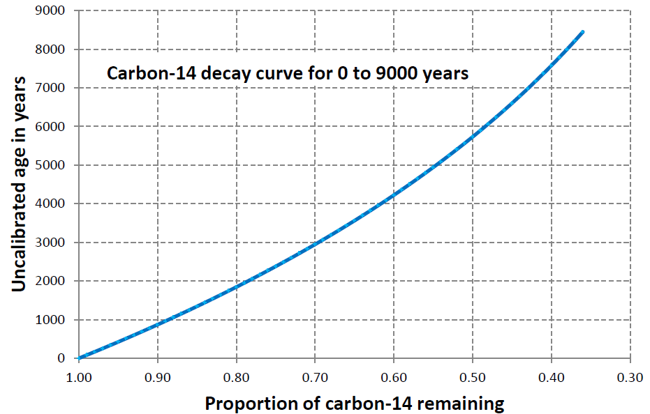
Exercise: Radiometric Dating with Potassium-Argon
Assume that a feldspar crystal from the granite shown in Figure 19.20 was analyzed for 40K and 40Ar. The proportion of 40K remaining is 0.91. Using the decay curve shown on this graph, estimate the age of the rock. An example is provided (in blue) for a 40K proportion of 0.95, which is equivalent to an age of approximately 96 Ma. This is determined by drawing a horizontal line from 0.95 to the decay curve line, and then a vertical line from there to the time axis.
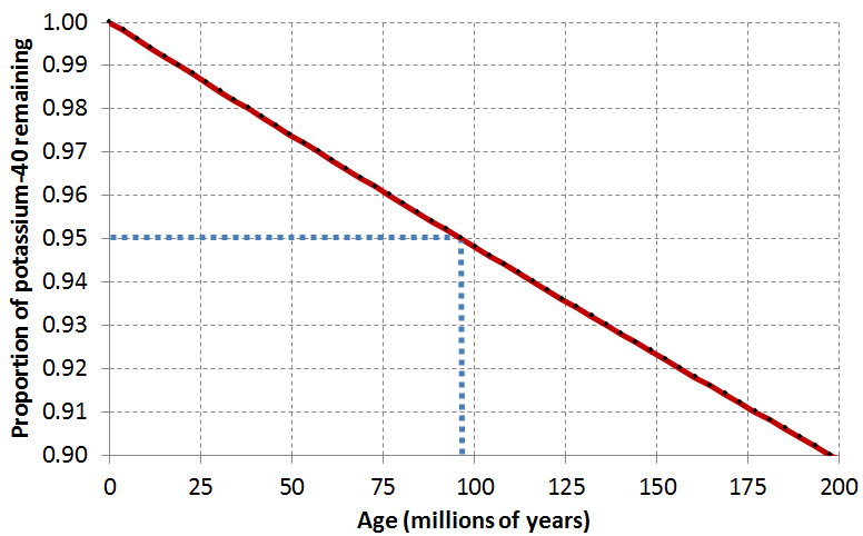_](figures/19-measuring-geological-time/figure-19-23.png)
Figure 19.25: Decay curve for potassium-argon dating. Source: Steven Earle (2015) CC BY 4.0 view source
19.5 Other Dating Methods
There are numerous other techniques for dating geological materials, but we will examine just two of them here: dendrochronology—tree-ring dating—and dating based on the record of reversals of Earth’s magnetic field.
19.5.1 Dendrochronology
Dendrochronology can be applied to dating very young geological materials based on reference records of tree-ring growth going back many millennia. The longest such records can take us back over 25 ka, to the height of the last glaciation. One of the advantages of dendrochronology is that, providing reliable reference records are available, the technique can be used to date events to the nearest year.
Dendrochronology has been used to date the last major subduction zone earthquake on the coast of B.C., Washington, and Oregon. When large earthquakes occur in this region, there is a tendency for some coastal areas to subside by one or two metres. Seawater then rushes in, flooding coastal flats and killing trees and other vegetation within a few months. There are at least four locations along the coast of Washington that have such dead trees, and probably many more in other areas. Wood samples from these trees have been studied and the ring patterns have been compared with patterns from old living trees in the region (Figure 19.26).
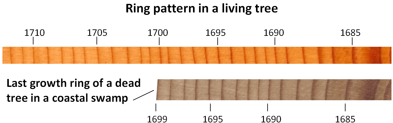_](figures/19-measuring-geological-time/figure-19-24.png)
Figure 19.26: Example of tree-ring dating of dead trees. Source: Steven Earle (2015) CC BY 4.0 view source
At all of the locations studied, the trees were found to have died either in the year 1699, or very shortly thereafter (Figure 19.27). On the basis of these results, it was concluded that a major earthquake took place in this region sometime between the end of growing season in 1699 and the beginning of the growing season in 1700. Evidence from a major tsunami that struck Japan on January 27, 1700, narrowed the timing of the earthquake to sometime in the evening of January 26, 1700. (For more information, see https://web.viu.ca/earle/1700-quake/.)
, from data in Yamaguchi et al. (1997)._](figures/19-measuring-geological-time/figure-19-25.png)
Figure 19.27: Sites in Washington where dead trees are present in coastal flats. The outermost wood of eight trees was dated using dendrochronology, and of these, seven died during the year 1699, suggesting that the land was inundated by water at this time. Source: Steven Earle (2015) CC BY 4.0 view source, from data in Yamaguchi et al. (1997).
19.5.2 Magnetic Chronology
Changes in Earth’s magnetic field can also be used to date events in geologic history. The magnetic field causes compass needles point toward the north magnetic pole, but this hasn’t always been the case. At various times in the past, Earth’s magnetic field has reversed its polarity, and during such times a compass needle would have pointed to the south magnetic pole. By studying magnetism in volcanic rocks that have been dated isotopically, geologists have been able to establish the chronology of magnetic field reversals going back for ~250 Ma. About 5 Ma of this record is shown in Figure 19.28, where the black bands represent periods of normal magnetism (“normal” meaning a polarity identical to the current magnetic field) and the white bands represent periods of reversed magnetic polarity. These periods of consistent magnetic polarity are given names to make them easier to reference. The current period of normal magnetic polarity, known as Brunhes, has lasted for the past 780,000 years. Prior to that there was a short reversed period and then a short normal period, the latter of which is known as Jaramillo.
_](figures/19-measuring-geological-time/figure-19-26.png)
Figure 19.28: The last 5 Ma of magnetic field reversals. Source: Steven Earle (2015) CC BY 4.0 view source, modified after U.S. Geological Survey (2007) Public Domain view source
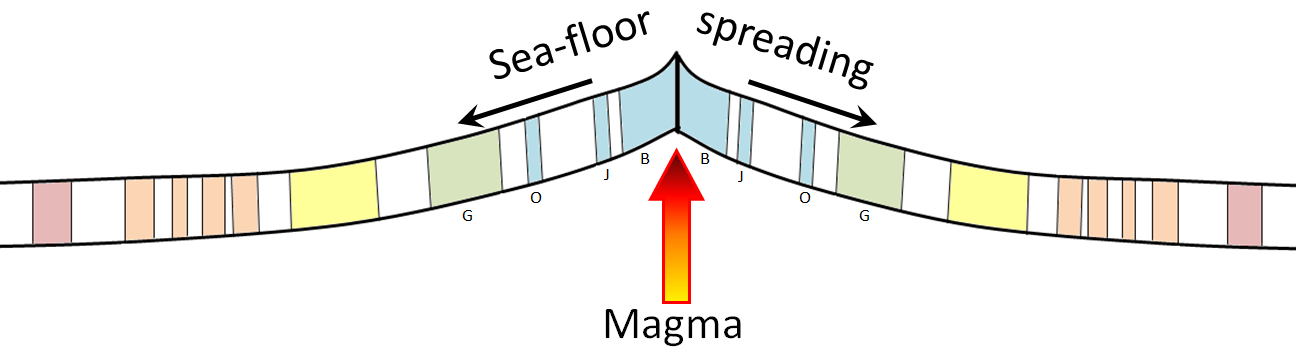
Oceanic crust becomes magnetized by the magnetic field that exists as the crust forms from magma at mid-ocean ridges. As it cools, the magnetic fields of tiny crystals of magnetite that form within the magma become aligned with the existing magnetic field, and remain in this orientation, even if Earth’s magnetic field later changes polarity (Figure 19.29). Oceanic crust that is forming today is being magnetized in a “normal” sense, but crust that formed 780,000 to 900,000 years ago, in the interval between the Brunhes and Jaramillo normal periods, was magnetized in the “reversed” sense.
_](figures/19-measuring-geological-time/figure-19-27.png)
Figure 19.29: Formation of magnetized oceanic crust at a spreading ridge. Coloured bars represent periods of normal magnetic polarity. Capital letters denote the Brunhes, Jaramillio, Olduvai, and Gauss normal magnetic periods (see Figure 19.28). Source: Steven Earle (2015) CC BY 4.0 view source
Magnetic chronology can be used as a dating technique because we can measure the magnetic field of rocks using a magnetometer, or of entire regions by towing a magnetometer behind a ship or an airplane. For example, the Juan de Fuca Plate, which lies off of the west coast of BC, Washington, and Oregon, is being and has been formed along the Juan de Fuca spreading ridge (Figure 19.30). The parts of the plate that are still close to the ridge exhibit normal magnetic polarity, while parts that are further away (and formed much earlier) have either normal or reversed magnetic polarity, depending upon when the rock formed. By carefully matching the sea-floor magnetic stripes with the known magnetic chronology, we can determine the age at any point on the plate. We can see that the oldest part of the Juan de Fuca Plate that has not yet subducted (off of the coast of Oregon) is just over 8 million years old, while the part that is subducting beneath Vancouver Island is between 0 and ~6 million years old.
_](figures/19-measuring-geological-time/figure-19-28.png)
Figure 19.30: TThe pattern of magnetism within the area of the Juan de Fuca Plate, off the west coast of North America. Coloured bands represent parts of the sea floor with normal magnetic polarity, and the magnetic time scale is shown using these same colours. Source: Steven Earle (2015) CC BY 4.0 view source
Exercise: Magnetic Dating
The fact that magnetic intervals can only be either normal or reversed places significant limits on the applicability of magnetic dating. If we find a rock with normal magnetism, we can’t know which normal magnetic interval it represents, unless we have some other information.
Using Figure 19.28 for reference, determine the age of a rock with normal magnetism that has been found to be between 1.5 and 2.0 Ma based on fossil evidence in nearby sedimentary rocks.
How old is a rock that is limited to 2.6 to 3.2 Ma by fossils, and which has reversed magnetic polarity?
19.6 Understanding Geological Time
It is one thing to know the facts about geological time — how long it is, how we measure it, how we divide it into smaller time intervals, and what we call the various periods and epochs — but it is quite another to really understand geological time. The problem is that our lives are short and our memories are even shorter. Our experiences span only a few decades, so we really don’t have a way of knowing what 11,700 years means. What’s more, it is hard for us to understand how 11,700 years differs from 65.5 Ma, or even from 1.8 Ga. It is not that we cannot comprehend what the numbers mean, it is that we cannot really appreciate how much time is involved.
You may wonder why it is so important to understand geological time. There are some very good reasons. One is so that we can fully understand how geological processes that seem impossibly slow can produce anything of consequence. Consider driving from one major city to another, where a journey of several hours might occur at speeds of ~100 km/h. Continents move toward each other at rates of a fraction of a millimetre per day, a speed something on the order of 0.00000001 km/h, and yet, at this impossibly slow rate (try walking at this speed!), they can move thousands of kilometres through geological time. Sediments typically accumulate at even slower rates — less than a millimetre per year — but still they are thick enough to be thrust up to form huge mountains or carved into breathtaking canyons.
Another reason is to understand issues like extinction of endangered species, and human influence on climate. People who do not understand geological time are quick to say that the climate has changed in the past, and that what is happening now is no different. And climate certainly has changed in the past: from the Eocene (50 Ma) to the present day, Earth’s climate cooled by ~12°C on average. This is a huge change that ranks as one of the most important climate changes of Earth’s past, and yet the rate of change over this time was only 0.000024 °C/century. Recent warming has occurred at a rate of ~1.1°C over the past 100 years (NASA GISS), 45,800 times faster than the rate of climate change since the Eocene.
One way to wrap your mind around geological time is to put it into the perspective of single year. At this rate, each hour of the year is equivalent to approximately 500,000 years, and each day is equivalent to 12.5 million years. If all of geological time is compressed down into a single year, Earth formed on January 1, and the first life forms evolved in late March (~3,500 Ma). The first multicellular life forms appeared on November 13 (~600 Ma), plants appeared on land on November 24, and amphibians on December 3. Reptiles evolved from amphibians during the first week of December, and dinosaurs and early mammals evolved by December 13. Non-avian dinosaurs, which survived for 160 million years, went extinct on Boxing Day (December 26). The Pleistocene glaciation began at ~6:30 p.m. on New Year’s Eve, and the last glacial ice melted from southern Canada by 11:59 p.m.
It is worth repeating: on this time scale, the earliest ancestors of the animals and plants with which we are familiar did not appear on Earth until mid-November, the dinosaurs disappeared after Christmas, and most of Canada was periodically locked in ice from 6:30 to 11:59 p.m. on New Year’s Eve. As for people, the first to inhabit Canada arrived about one minute before midnight.
Exercise: What Happened on Your Birthday?
Using the “all of geological time compressed to one year” concept, determine the geological date that is equivalent to your birthday. First, go hereto find out which day of the year your birth date is. Divide that number by 365, and multiply that number by 4,570 to determine the time (in millions since the beginning of geological time). Subtract that number from 4,570 to determine the date back from the present.
Example: April Fool’s Day (April 1) is day 91 of the year: 91/365 = 0.2493. 0.2493 x 4,570 = 1,139 million years from the start of time, and 4,570 - 1,193 = 3,377 Ma is the geological date.
Finally, go to the Foundation for Global Community’s Walk through Time website to find out what was happening on your day. The nearest date to 3,377 Ma is 3,400 Ma.
19.7 Summary
The topics covered in this chapter can be summarized as follows:
19.7.1 The Geological Time Scale
The work of William Smith was critical to the establishment of the first geological timescale early in the 19th century, but it wasn’t until the 20th century that geologists were able to assign reliable dates to the various time periods. The geological timescale is now maintained by the International Commission on Stratigraphy. Geological time is divided into eons, eras, periods, and epochs.
19.7.2 Relative Dating Methods
We can determine the relative ages of different rocks by observing and interpreting relationships among them, such as superposition, cross-cutting, and inclusions. Gaps in the geological record are represented by various types of unconformities.
19.7.3 Dating Rocks Using Fossils
Fossils are useful for dating rocks back to ~600 Ma. If we know the age range of a fossil, we can date the rock in which it is found, but some organisms lived for many millions of years. Index fossils represent shorter geological time spans, and if a rock has several different fossils with known age ranges, we can narrow the time during which the rock formed.
19.7.4 Isotopic Dating Methods
Radioactive isotopes decay at constant known rates, and can be used to date igneous and metamorphic rocks. Some commonly used isotope systems are potassium-argon, rubidium-strontium, uranium-lead, and carbon-nitrogen. Radiocarbon dating can be applied to sediments and sedimentary rocks, but only if they are younger than 60 ka, and contain organic material, or minerals of calcium carbonate.
19.7.5 Other Dating Methods
There are many other methods for dating geological materials. Two that are widely used are dendrochronology and magnetic chronology. Dendrochronology, based on studies of tree rings, is widely applied to dating glacial events. Magnetic chronology is based on the known record of Earth’s magnetic field reversals.
19.7.6 Understanding Geological Time
While understanding geological time is relatively easy, actually comprehending the significance of the vast amounts of geological time is a great challenge. To be able to solve important geological problems and certain societal challenges, we need to really appreciate the vastness of geological time.
19.8 Chapter Review Questions
A granitic rock contains inclusions (xenoliths) of basalt. What can you say about the relative ages of the granite and the basalt?
Explain the differences between a) disconformity and paraconformity; and b) nonconformity and angular unconformity
What are the features of a useful index fossil?
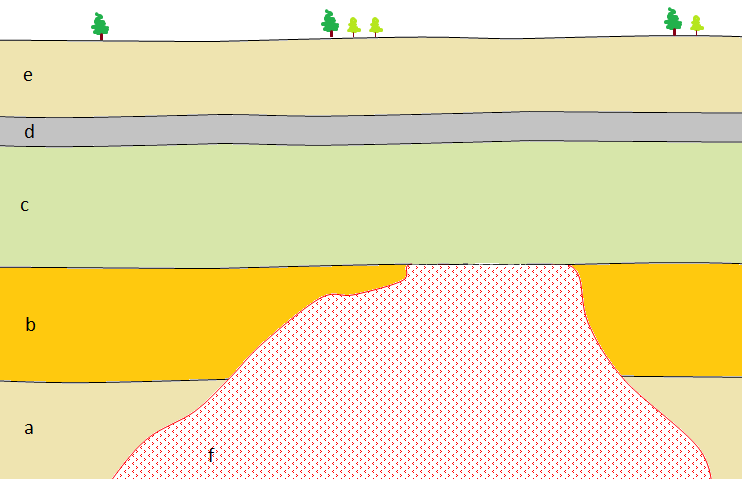
Figure 19.31 shows a geological cross-section. The granitic rock F at the bottom is the rock that you estimated the age of in the exercise in 19.4, Radiometric Dating with Potassium-Argon. A piece of wood from layer D has been sent for radiocarbon dating and the result was 0.55 14C remaining. How old is layer D?
Based on your answer to question 4, what can you say about the age of layer C in the figure above?
What type of unconformity exists between layer C and rock F?
What type of unconformity exists between layer C and rock B?
We cannot use magnetic chronology to date anything older than ~780,000 years. Why?
How did William Smith apply the principle of faunal succession to determine the relative ages of the sedimentary rocks of England and Wales?
Access a copy of the geological time scale at http://www.stratigraphy.org/index.php/ics-chart-timescale. What are the names of the last age of the Cretaceous and the first age of the Paleogene? Print out the time scale and stick it on the wall above your desk!
. Right- Steven Earle (2015) CC BY 4.0 [view source](http://opentextbc.ca/geology/wp-content/uploads/sites/110/2015/07/diagram.png)_](figures/19-measuring-geological-time/figure-19-29.png)
Figure 19.31: Geological cross-section (left) and decay curve for 14C ages. Source: Left- Karla Panchuk (2018) CC BY 4.0, modified after Steven Earle (2015) CC BY 4.0 view source. Right- Steven Earle (2015) CC BY 4.0 view source
19.9 Answers to Chapter Review Questions
Xenoliths of basalt within a granite must be older than the granite according to the principle of inclusions.
- At both disconformities and paraconformities the beds above and below are parallel, but at a disconformity there is clear evidence of an erosion surface (the lower layers have been eroded). (b) A nonconformity is a boundary between sedimentary rocks above and non-sedimentary rocks below while an angular unconformity is a boundary between sedimentary rocks above and tilted and eroded and sedimentary layers below.
A useful index fossil must have survived for a relatively short period (e.g., around a million years), and also should have a wide distribution so that it can be used to correlate rocks from different regions.
The granitic rock F has been dated to 175 Ma. The wood in layer D is approximately 5,000 years old, so we can assume that layer D is no older than that, although it could be as much as a few hundred years younger if the wood was already old when it got incorporated into the rock.
Layer C must be between 5,000 y and 275 Ma.
The unconformity between layer C and rock F is a nonconformity.
The granite (F) was eroded prior to deposition of C, so it’s likely that layer B was also eroded at the same time. If so, that makes the boundary between C and B a disconformity.
The last magnetic reversal was 780,000 years ago, so all rock formed since that time is normally magnetized and it isn’t possible to distinguish older rock from younger rock within that time period using magnetic data.
William Smith was familiar with the different diagnostic fossils of the rocks of England and Wales and was able to use them to identify rocks of different ages.
The last age of the Cretaceous is the Maastrichtian (71.2 to 66.0 Ma) and the first age of the Paleogene is the Danian (66.0 to 61.6 Ma).
19.10 References
Smith, W. (1815). A delineation of the strata of England and Wales with part of Scotland [map].
Harries, P.J., Kauffman, E.G., Crampton, J.S. (Redacteurs), Bengtson, P., Cech, S., Crame, J.A., Dhondt, A.V., Ernst, G., Hilbrecht, H., Lopez, Mortimore, G.R., Tröger, K.-A., Walaszcyk, I., & Wood, C.J. (1996). Mitteilungen aus dem Geologisch - Paläontologischen Museum der Universität Hamburg, 77, 641-671.Full text
Scott, R. (2014). A Cretaceous chronostratigraphic database: construction and applications, Carnets de Géologie, 14(2), 15-37. Full text
Clague, J. (1976). Quadra Sand and its relation to late Wisconsin glaciation of southeast British Columbia. Canadian Journal of Earth Sciences, 13, 803-815.
Yamaguchi, D.K., Atwater, B.F., Bunker, D.E., Benson, B.E., & Reid, M. S. (1997). Tree-ring dating the 1700 Cascadia earthquake. Nature, 389, 922 - 923.
NASA Goddard Institute for Space Studies (n.d.). GLOBAL Station Temperature Index in 0.01 degrees Celsius base period: 1951-1980 [data file]. Retrieved from http://data.giss.nasa.gov/gistemp/tabledata_v3/GLB.Ts.txt